- Review
- Open access
- Published:
Maritime continent coastlines controlling Earth’s climate
Progress in Earth and Planetary Science volume 5, Article number: 21 (2018)
Abstract
During the Monsoon Asian Hydro−Atmosphere Scientific Research and Prediction Initiative (MAHASRI; 2006–16), we carried out two projects over the Indonesian maritime continent (IMC), constructing the Hydrometeorological Array for Intraseasonal Variation−Monsoon Automonitoring (HARIMAU; 2005–10) radar network and setting up a prototype institute for climate studies, the Maritime Continent Center of Excellence (MCCOE; 2009–14). Here, we review the climatological features of the world’s largest “regional” rainfall over the IMC studied in these projects. The fundamental mode of atmospheric variability over the IMC is the diurnal cycle generated along coastlines by land−sea temperature contrast: afternoon land becomes hotter than sea by clear-sky insolation before noon, with the opposite contrast before sunrise caused by evening rainfall-induced “sprinkler”-like land cooling (different from the extratropical infrared cooling on clear nights). Thus, unlike the extratropics, the diurnal cycle over the IMC is more important in the rainy season. The intraseasonal, seasonal to annual, and interannual climate variabilities appear as amplitude modulations of the diurnal cycle. For example, in Jawa and Bali the rainy season is the southern hemispheric summer, because land heating in the clear morning and water vapor transport by afternoon sea breeze is strongest in the season of maximum insolation. During El Niño, cooler sea water surrounding the IMC makes morning maritime convection and rainfall weaker than normal. Because the diurnal cycle is almost the only mechanism generating convective clouds systematically near the equator with little cyclone activity, the local annual rainfall amount in the tropics is a steeply decreasing function of coastal distance (e-folding scale 100–300 km), and regional annual rainfall is an increasing function of “coastline density” (coastal length/land area) measured at a horizontal resolution of 100 km. The coastline density effect explains why rainfall and latent heating over the IMC are twice the global mean for an area that makes up only 4% of the Earth’s surface. The diurnal cycles appearing almost synchronously over the whole IMC generate teleconnections between the IMC convection and the global climate. Thus, high-resolution (<< 100 km; << 1 day) observations and models over the IMC are essential to improve both local disaster prevention and global climate prediction.

Introduction
Tropical rainfall in the global climate
Recognition of rainfall as one of the most important quantities for classifying climate and its global quantitative description was established by Köppen (1918), who divided the tropical climate (A; classified by temperature in his first world climate map in 1884) into rainforest (Af) and the savanna (Aw), according to vegetation. This is also physically reasonable, because in essence, the temperature and rainfall represent the sensible (radiative) and latent heating processes, respectively, that maintain the climate (Fig. 1a). Note that rainfall is a flux quantity (amount per area per time) dependent on horizontal and temporal scales (such as the hourly, daily, monthly, and annual rainfall measured by a single-station rain gauge, in a radar-observed area, and over an integrated region) and that it fluctuates greatly because individually short-lived small precipitating clouds are organized into multiple scale structures. In this article, we consider mainly a “regional” rainfall with a scale somewhat larger than that supposed (seasonal−annual and 102–103 km) by Köppen on the basis of vegetation.

a The global energy and water cycle (modified from Trenberth et al. 2009) and its alternative distributions: b in sea and land (modified from Hartmann 1994, with values according to Trenberth et al. 2009) and c in latitude (modified from Hartmann 1994, which was based on Baumgartner and Reichel 1975; originally much older, at latest up to Meinardus’ analysis published in 1934; see Jaeger 1983). d Low-latitude part of Köppen’s (1918) original climate classification map showing already both latitudinal and coastal dependencies
Köppen classified low latitude regions of South America and Africa and most of the “East Indies” as Af climate regions defined by a minimum monthly rainfall ≥ 60 mm/month (total annual rainfall >> 720 mm/year), but carefully excluded the inland areas of Sumatera, Kalimantan and Papua,Footnote 1 as well as those of South America and Africa (except for the Amazon and Congo River Basins) so that his “idealized” land had Af along the equator including inland areas (see Fig. 1d). This view of the rainfall concentration in the equatorial coastal areas was still accepted after some revisions up to his updated version (Köppen and Geiger 1954),Footnote 2 but is no longer consistent with recent descriptions (Peel et al. 2007).Footnote 3 The smaller (Lesser Sunda) islands between Jawa and Papua were also excluded from Af, which was recognized as a west−east difference in the Indonesian maritime continent (IMC). At present, a detailed gridded rainfall distribution based on rain gage data (APHRODITE; Yatagai et al. 2012) shows differences between coastal and inland regions, although this is less clear than in the space-borne radar data to be mentioned later.
Köppen’s son-in-law Wegener (1929, after revisions of the first edition published in 1915) tried to use his father-in-law’s idealized climate distribution (1918) to estimate the geographical location of his proposed early-Mesozoic supercontinent before separation and drift, assuming the Af climate near the equator and the coastline. He also speculated on the origin of the East Indies by the association of northward movement of the Indian subcontinent followed by the Australian continent, which is essentially consistent with present-day plate tectonics after a long period of controversy (e.g., Frankel 2012). Köppen and Wegener (1924) evaluated the importance of theories of climate variability associated with insolation changes, developed by Milanković, a Serbian applied mathematician, who published a compilation of these theories (Milanković 1941), which concerned mainly long-term historical climate change (ice ages) but were based on the variation of insolation with the axis of the Earth’s rotation that will be described later in this article. The East Indies, that is the present-day Indonesian Archipelago, and surroundings were designated the maritime continent by Ramage (1968), based on the occurrence frequency of thunderstorms, which was the only database covering the whole equatorial region at that time. In the tropics, thunderstorms as well as rainfall are dependent on convective cloud activity, and the Indonesian maritime continentFootnote 4 (hereafter referred to as IMC) is known as the world’s convection center or the region of maximum rainfall on Earth.
The IMC was one of the most important regions for hydroclimate studies during the Monsoon Asian Hydro−Atmosphere Scientific Research and Prediction Initiative (MAHASRI; 2006–2016) and the Asian Monsoon Years (AMY; 2007–2012)Footnote 5 in the World Climate Research Programme (WCRP) (Matsumoto et al. 2016, 2017; Yamanaka et al. 2016). This is simply because the IMC is the region with the world’s largest regional rainfall but has no sufficiently reliable observation network. In the subsequent two subsections we summarize the scientific background and implementation of the two projects carried out over the IMC related to MAHASRI and AMY.
The global energy/water cycle and the maritime continent
The Earth’s climate system includes latent heat input from the ground to the atmosphere through the cloud−precipitation process (Fig. 1a), which is also a part of the water cycle between the land and ocean through the atmosphere (Fig. 1b). The meridional peak of the cloud−precipitation activity (corresponding to rainfall amounts of about 2000 mm/year ≈ 5.5 mm/day) is located in the tropics along the equator (Fig. 1c). The equatorial rainfall peak is consistent with the intertropical convergence zone (ITCZ) in the general circulation (Fig. 2a) known since Halley’s (1686) observations and Hadley’s (1735) theory.Footnote 6 It is surprising that the maximum value was known rather correctly more than a century ago (cf. Jaeger 1983), when stations were restricted to major cities over land, in particular along the coastlines.

Schematic diagrams of distributions of tropical precipitation: a simple ITCZ as considered by Hadley in 18th century, b MJOs propagating eastward as simulated in an “aqua planet” model (e.g., Hayashi and Sumi 1986), and c concentration along coastlines as described in this article
Geographical rainfall distributions with the meridional peak around 2000 mm/year in the tropics are estimated also from satellite cloud observationsFootnote 7 and simulated by numerical climate models, for example, as shown in a report of the Intergovernmental Panel on Climate Change (IPCC) (Randall et al. 2007) (Fig. 3), although peak values are somewhat larger than the direct rainfall observations from rain gages and radars. An IPCC-related study (Yoshida et al. 2005) has compared these estimates and their simulations (the Community Climate System Model version 3 (CCSM3) model; Collins et al. 2006) of the mean annual rainfall amounts in various regions, of which 10 are inside the tropics (see the two columns labeled IPCC07 in Table 1). The IMC is the region of the most active convective clouds producing the largest regional rainfall on Earth (around 2700 mm/year ≈ 7 mm/day). The second highest regional rainfall is found in Central America.

a, b Rainfall distributions a “observed” and b simulated for IPCC AR4 (Randall et al. 2007)
The world’s largest regional rainfall over the IMC has often been explained in terms of the warmest seawater surrounding the IMC (Fig. 4b), which looks just like a “dam” for the global “river” of Indonesian throughflow from the Pacific to the Indian Ocean (e.g., Lukas et al. 1996; Gordon 2005). However, rainfall over the open ocean including the ITCZ is less than that over the islands in the IMC. The tropical atmosphere is conditionally unstable; convection is developed only when cloud appears, whereas a cloud is generated when convection develops. This paradoxical situation may be overcome over the open ocean by conditional instability of the second kind (CISK), which generates tropical cyclones in the subtropics and intraseasonal variations (ISVs) along the equator (Ooyama 1971; Lindzen 1974; Hayashi and Sumi 1986). Tropical cyclones generally appear outside the IMC. The ISVs (shown in Fig. 2b), which often have the so-called Matsuno−Gill pattern (Matsuno 1966; Gill 1980), are actually dominant and known as the Madden−Julian oscillations (MJOs) over the open ocean (Madden and Julian 1971, 1994; Nakazawa 1988; Zhang 2005, 2013; Yoneyama et al. 2008, 2013) on both the western and the eastern sides of the IMC (Fig. 5). However, such transient or traveling disturbances are modified or weakened on reaching the IMC (Nitta et al. 1992; Hashiguchi et al. 1995; Widiyatmi et al. 2001; Sakurai et al. 2005; Shibagaki et al. 2006; Hidayat and Kizu 2010; Marzuki et al. 2013) and cannot explain the convective clouds and rainfall over the IMC throughout the year.


ISVs arriving at the IMC a around the time of rainy season onset (November–December 1992) observed by a wind profiler (12 h averaged) at Serpong (6° S, 107° E) (left) and a GMS (hourly) Hovmöller diagram along 6° S (right) (Hashiguchi et al. 1995) and b during a rainy season (December 2007) by a wind profiler network at Kototabang (0° S, 100° E), Pontianak (0° S, 110° E), and Biak (1° S, 136° E) (map and left three panels) and GMS along the equator (right) (Yamanaka et al. 2008), showing modification/decay (smaller hierarchies associated with reversals in profiler zonal winds) mainly due to the diurnal cycle (appearing in GMS clouds) over the IMC
On the other hand, the land is heated more easily than the sea (Fig. 4a), but convective clouds generated over the true continents (Africa and South America) are less active than those over the IMC. Therefore, another systematic mechanism is necessary to kick-off an initial updraft in the conditionally unstable tropical atmosphere, and it must work most actively over the IMC.
We have also noticed climatic variabilities of the IMC (cf. Yamanaka 2016): two systematic periodical (annual and diurnal) cycles that are forced astronomically and other components without fixed periodicity (ISVs and interannual variations). The annual cycles of rainy (monsoon) and dry seasons are less clear in the IMC than in adjacent regions such as Indochina (Murakami and Matsumoto 1994) and vary spatially: the seasonal march in the southern hemispheric part (Jawa and Bali) has a southern-hemispheric annual cycle (a clear rainfall maximum in southern summer) (e.g., Haylock and McBride 2001; Hamada et al. 2002; Aldrian and Susanto 2003; McBride et al. 2003; Chang et al. 2004, 2016). The equatorial and northern-hemispheric parts have either a semi-annual cycle (with double peaks near equinox seasons), a northern-hemispheric annual cycle (one peak in northern summer), or the cycle is unclear. The semi-annual cycle is reasonable if we consider that the sun passes the zenith, when the insolation becomes maximum, twice a year. So the rainfall over the IMC is sensitive to the insolation. However, why is the insolation stronger in the rainy and cloudy season? Why is the southern-hemispheric rainy season so dominant in low-latitude Jawa and Bali? We must answer these questions adequately, as well as establishing the mechanism to explain why the world’s largest regional rainfall falls over the IMC.
JEPP−HARIMAU and SATREPS−MCCOE projects
Our observations have been outlined in Yamanaka et al. (2008, 2016) and Yamanaka (2016), and here, we give some details of the background (see also the map in Fig. 5b). The most important aspect in promoting a hydroclimate project over Southeast Asia in the present century is that both infrastructure and the need for observations have grown rapidly with economic growth. More complete understanding and more accurate predictability are requested strongly from industry and the public sectors that have graduated quickly from day-to-day business and a hand-to-mouth existence. The numbers of universities and their students are also increasing rapidly. These circumstances have encouraged governments to promote hydroclimatology with resolution better than annual or continental scale monsoons, as well as with interannual and global scope to maintain sustainable development by mitigating the effects of climate change. Therefore, scientific studies have been conducted in parallel with projects for societal applications (e.g., disaster prevention) and capacity building.
Projects related to MAHASRI and AMY over the IMC are most typical in view of their relevance to the criteria mentioned above. In particular, high-resolution radar observations were strongly requested by both hydroclimatological interest in the world’s strongest convective activity and the societal impacts such as frequent flood and landslide disasters. When we proposed a project related to MAHASRI over the IMC, the Japanese Government established the Japan Earth-Observation System Promotion Program (JEPP) contributing to the Global Earth Observation System of Systems (GEOSS; see GEO 2007), which emphasized societal benefits. Our proposal for the Hydrometeorological ARray for Intraseasonal variation−Monsoon AUtomonitoring (HARIMAU) (Yamanaka et al. 2008)Footnote 8 was approved as a JEPP project and was conducted from August 2005 to March 2010 (see: http://www.jamstec.go.jp/iorgc/harimau/HARIMAU.html), in collaboration with the Japan Agency for Marine−Earth Science and Technology (JAMSTEC), Kyoto University, Hokkaido University, the Agency for the Assessment and Application of Technology (BPPT), the Indonesian National Institute of Aeronautics and Space (LAPAN), and the Indonesian Agency for Meteorology, Climatology and Geophysics (BMKG). HARIMAU consisted of a radar-profiler network with meteorological Doppler radars of X-band (at Padang; e.g., Kawashima et al. 2011; Mori et al. 2011; Sakurai et al. 2011; Kamimera et al. 2012) and C-band (at Serpong near Jakarta; e.g., Wu et al. 2013; Mori et al., 2018, personal communication), and wind profilers of L-band (at Pontianak, Manado, and Biak; e.g., Tabata et al. 2011a, 2011b). A large very high frequency (VHF) wind profiler called the Equatorial Atmosphere Radar (EAR) located at Kototabang (e.g., Fukao 2006; Shibagaki et al. 2006; Seto et al. 2009) was also included in the network. Rainfall and wind distribution data were displayed via the Internet in near real-time throughout the project.
Since 2005, the Indonesian Government has funded the BMKG’s efforts to install over 40 meteorological radars.Footnote 9 The number of radiosonde stations was also increased to 22, which contributed to the improved accuracy of objective analyses at meteorological agencies worldwide (cf. Seto et al. 2009).Footnote 10 In parallel with the measurements obtained by the radars and radiosondes, JAMSTEC and BPPT collaborated on buoy and shipboard observations over the Indonesian exclusive economic zone (EEZ) as part of the international network of the Tropical Ocean Climate Study (TOCS; Ando et al. 2010). Another JEPP project, the Indian Ocean Moored Network Initiative for Climate Studies (IOMICS), collected data during 2005–2010 as part of the Research Moored Array for African−Asian−Australian Monsoon Analysis and Prediction (RAMA; McPhaden et al. 2009). Ship-based sea water, surface weather, radar, and radiosonde observations on atmosphere−ocean interactions over the Indian Ocean were conducted by the Mirai Indian Ocean Cruise for the Study of the MJO−Convection Onset in 2006 (MISMO2006; Yoneyama et al. 2008).
In 2009, a follow-on project to HARIMAU and IOMICS was approved under the Science and Technology Research Partnership for Sustainable Development (SATREPS). This project established an international center of tropical climatology, meteorology, and oceanography, called the Maritime Continent Center of Excellence (MCCOE) under BPPT in November 2013 and included capacity building for radar operations and buoy manufacturing during February 2010–March 2014 (see http://www.jamstec.go.jp/rigc/tcvrp/satreps_id/ in Japanese). Some observations were conducted also in collaboration with the Cooperative Indian Ocean Experiment on Intraseasonal Variability in the Year 2011 (CINDY2011; Yoneyama et al. 2013). After MCCOE was established, the HARIMAU radars and profilers came under the responsibility of that center. Observational data have contributed to global reanalysis (e.g., Onogi et al. 2007; Kobayashi et al. 2015), as well as high-resolution numerical studies at both regional (e.g., Wu et al. 2008, 2009) and global (e.g., Sato et al. 2009) scales.
The HARIMAU campaign observations were carried out during periods of intense observation almost every year from 2006 to 2011, under a collaboration with MAHASRI and other international projects (Table 2). In particular, HARIMAU2006, 2007 and 2011 were in the westernmost area of the IMC (Propinsi Sumatera Barat or West Sumatra Province), targeting the MJOs from the Indian Ocean and their modification (Yoneyama et al. 2008, 2013; Kamimera et al. 2012; Kubota et al. 2015, with the MISMO and CINDY projects), the diurnal cycles of the major and smaller islands (Wu et al. 2008, 2009; Kamimera et al. 2012), and convective cloud structure and vertical coupling (Fukao 2006; Mori et al. 2011; Kawashima et al. 2006, 2011; Sakurai et al. 2009, 2011, with the Coupling Processes in the Equatorial Atmosphere (CPEA) project). HARIMAU2008 and 2009 were performed over Kalimantan Island (Wu et al. 2008, 2009). HARIMAU2010 focused on the JABODETABEK (Jakarta−Bogor−Depok−Tangerang−Bekasi, or greater Jakarta) area, in collaboration with a hydrological study of the Ciliwung River (Sulistyowati et al. 2014; Mori et al., 2018, personal communication; Katsumata et al., 2018, personal communication).
Many other projects over this important region have been carried out in collaboration with various countries and agencies, for example, ocean–atmosphere interaction studies with China (e.g., Yang et al. 2015), aerosol studies with the USA and others (e.g., Reid et al. 2016), a collaboration within Southeast Asia (e.g., Koh and Teo 2009), and a collaboration/capacity building for meteorological operations and database construction with Australia, the Netherlands, France, Germany, and others. Collaborations between projects are occurring, and contributions from Indonesian scientists are increasing (see the last paragraph of the “Conclusions” section of this article).
In this article, we review mainly our own observational studies on the mechanisms generating the world’s largest regional rainfall over the IMC under the JEPP−HARIMAU and SATREPS−MCCOE projects. The “Review” section is separated into five subsections. The “Diurnal cycle observed around the IMC coastlines” section concerns observational evidence of the diurnal cycle near coastlines, which is the most fundamental and dominant mode over the IMC. The “Local rainfall as a function of coastline length” section describes the general feature of tropical rainfall concentration near coastlines. The “Regional rainfall as a function of ‘coastline density’” section explains the largest regional rainfall over the IMC in terms of the concentration of coastal diurnal cycle rainfall. The “Consistency with the global water budget” section estimates the contribution of the IMC rainfall to the global water/energy cycle. The “Control of the global climate” section looks toward connections between the IMC rainfall and the global climate.
Review
Diurnal cycle observed around the IMC coastlines
The dominant periodicity of insolation is diurnal, and sea−land heat capacity contrasts enforce the local diurnal variations in wind, clouds, and rainfall that were known in Batavia (now Jakarta) a century ago (van Bemmelen 1922). These diurnal variations have been confirmed everywhere along the coastal zones of larger islands (Sumatera, Kalimantan, Jawa, Sulawesi, and Papua) of the IMC, based on wind profilers (including raindrop measurements) (e.g., Hashiguchi et al. 1995; Renggono et al. 2001; Hadi et al. 2002; Murata et al. 2002; Araki et al. 2006; Marzuki et al. 2009; Tabata et al. 2011b), precipitation radars (e.g., Kawashima et al. 2006, 2011; Wu et al. 2007, 2013; Sakurai et al. 2009, 2011; Mori et al. 2011; Kamimera et al. 2012), a space-borne precipitation radar (e.g., Sorooshian et al. 2002; Mori et al. 2004; Kikuchi and Wang 2008; Wu et al. 2008, 2009; Peatman et al. 2014), GPS radio occultation (precipitable water or moisture) sounding (e.g., Wu et al. 2003, 2008, 2009), and satellite observations of outgoing longwave (infrared) radiation (OLR) (cloud-top temperature or height) (e.g., Hendon and Woodberry 1993; Nitta and Sekine 1994; Ohsawa et al. 2001; Yang and Slingo 2001; Sakurai et al. 2005; Hamada et al. 2008). As categorized by Kikuchi and Wang (2008), the diurnal cycle over the IMC is different from that over the open ocean (e.g., Sui et al. 1997).
Figure 6 shows examples of monthly averages of hourly OLR (cloud top temperature) observations by a Geostationary Meteorological Satellite (GMS) over the IMC and surrounding oceans. Individual mesoscale diurnal cycles are generated almost synchronously along coastlines of the archipelago, so that the whole (synoptic scale) IMC oscillates with an almost uniform diurnal cycle, which is consistent with the coastal heavy rainband organization previously reported (e.g., Mori et al. 2004, 2011, (2018, personal communication). We have carried out spectral analyses of the GMS data accumulated for 14 years over the IMC−Pacific region (Fig. 7a, the same region as Fig. 6). Geographical distributions of the frequency power-spectral density for selected components are plotted in Fig. 7b. This clearly shows the primary dominance of diurnal cycles and the secondary importance of annual cycles around major islands of the IMC and surrounding tropical regions. The diurnal cycle is particularly clear just on the landward side of the coastline, whereas the annual cycle appears somewhat vaguely and mainly inland. Figure 7c, d, are examples of frequency and zonal wavenumber spectral analyses. In the frequency domain, a striking spectral line corresponding to the diurnal cycle and the shorter period red noise-like continuum spectrum (to its right) are both stronger around the IMC than over the ocean. The wavenumber domain is only continuum-spectral (except for a flection around 300 km in wavelength, which will be mentioned later). These panels confirm that spatially broad-band (meso-to-synoptic scale) convection is the end result of the diurnal cycle energy input, although intermediate nonlinear processes may play a role and should be investigated further.

Monthly-mean 3-hourly GMS cloud-top height (temperature) distributions in 1999. The analyzed region is shown in a map in Fig. 7a. Time is in JST (= LT +2 h)

Spectral analysis of 14-year (1996–2009) hourly GMS−OLR cloud top temperature for the region a (Yamanaka 2016). Frequency spectra are b plotted geographically for 6 h to 2-year components and are shown c for five locations at every 20° longitude from 100° to 180° E along the equator (indicated by stars in a). d Zonal wavenumber spectra for the 90° E–150° W longitude range at every 5° latitude around the equator
Figure 8b, e show the mean annual rainfall (over a period of about 13 years; Ogino et al. 2016) and the local AM−PM rainfall difference (for 3 years; Mori et al. 2004) over the IMC, analyzed from space-borne precipitation radar (PR) data from the Tropical Rainfall Measurement Mission (TRMM) satellite. Rainfall amount is large near the coastlines, and morning (evening) rainfall is concentrated over the sea (land) side of a coastline. In central Africa (Fig. 8a, d) and South America (Fig. 8c, f), there are major inland rainfall regions, but circular distributions of rainfall amount and AM−PM difference are found, albeit faintly, around the Congo and Amazon river basins (which will be discussed later), in addition to remarkable coastal diurnal cycle rainfall areas over the Gulf of Guinea and Lake Victoria (as well as the Gulf of Panama, although this lies outside Fig. 8f). Hirose et al. (2017) show much higher resolution analyses including smaller island features and even a land–large river contrast over the Amazon River.

a−c annual amount (analyzed for Dec 1997−Jan 2011; Ogino et al. 2016) and d−f AM−PM difference (Jan 1998−Dec 2000; Mori et al. 2004) of rainfall for a, d central Africa, b, e South/Southeast Asia, and c, f South America observed by the TRMM-PR. Circles in d, f indicate rough locations of the contour line around which the mountain valley breeze circulation occurs
Figure 9a shows an example of frequency spectra of temperature at the surface and near the tropopause observed by radiosondes launched three hourly from both sides of a coastline near Bengkulu, southwestern Sumatera. Figure 9b, c show mean diurnal variations of the land and marine atmosphere temperature for the lowest 1 km obtained by the radiosonde observations. The diurnal cycle of temperature is striking near the land surface below about 300 m but is weak near the tropopause in spite of the cloud top height having a clear diurnal cycle. In particular, for the lowest 100 m on land, the lapse rate is large in the daytime (below 40 m, each temperature profile is often partly super-adiabatic, hence absolutely unstable around 06 UT = 13 LT), whereas it is negative (that is an inversion, i.e., strongly stable) in the nighttime 15−24 UT (22−07 LT).

Examples of a frequency power spectra (at a coastal land station in Bengkulu (04°S, 102°E), southwestern coast of Sumatera); b, c 10 day-mean land (Bengkulu)/marine (RV Mirai, approximately 50 km SW from Bengkulu) atmospheric temperature diurnal cycles below 1 km altitude; and d their difference, obtained during 8–18 December 2015. The abscissas of b−d are in UT (= LT−7 h). Details of the observations are described in Yokoi et al. (2017) and Wu et al. (2018)
Actual surface temperature is determined by complex boundary layer processes of radiation, convection (with eddy motion on smaller scales than the cloud convection) and conduction (molecular properties, less important than the other two in the atmosphere, except just above the surface) interacting with each other (e.g., section 14.1 in Stull 1988). For example, if clouds are generated by surface heating in daytime, the heating becomes immediately reduced by the albedo (parasol effect) of the clouds. Rainfall produced by the clouds on land in nighttime cools down the land surface temperature like a sprinkler (Fig. 10b; Wu et al. 2009), as shown observationally in Fig. 9b and numerically in a global high-resolution model (Sato et al. 2009). As a result, there is almost no “tropical night”Footnote 11 in the tropics (Fig. 10b). This sprinkler-like self-cooling process is different from the extratropical diurnal cycle that needs radiative cooling in clear weather through day and night. Thus, over the IMC, the latent heat and the sprinkler-like effect should have comparable magnitudes with the other (sensible or radiative) heating or cooling mechanisms such as insolation, infrared radiation, and the greenhouse effect. Hadi et al. (2002) and Araki et al. (2006) presented climatological analyses of diurnal cycles near Jakarta in northwestern Jawa and discussed differences between dry and rainy seasons and between wind and rainfall.

a Mean annual cycle of the monthly maximum insolation at Serpong (6° S, 107° E) near Jakarta during 1993–2002 (Araki et al. 2006), b monthly temperature variation at Pontianak (0°, 109° E), west Kalimantan in April 2002 (Wu et al. 2008), and c mechanism (Wu et al. 2009) of the diurnal cycle over the IMC
Usually the land surface, which has a smaller effective heat capacity, is heated or cooled by any thermal forcing more quickly and more largely than the sea surface with larger effective heat capacity, and the horizontal gradient (sea−land difference) of surface temperature (precisely, atmospheric bottom temperature) directly governs the amplitude of diurnal cycles (e.g., Kimura 1975; Rotunno 1983; Niino 1987; Niino et al. 2006). Figure 9d shows mean diurnal variations of the land−sea atmosphere temperature difference for the lowest 1 km obtained by radiosonde observations. Warmer land than sea is observed through the analyzed altitude range (especially strong below 500 m) during daytime (10−16 LT, with a downward phase delay), whereas sea is warmer than land by a greater amount and for longer (19−07 LT) but only below 200-m altitude. This asymmetric temperature cycle seems consistent with the diurnal cycle rainfall being heavier in the morning on the sea-side than in the evening on the land-side (contrary to the cloud top height shown in Fig. 6) as observed in various coastal areas (Sumatera, Jawa, and Kalimantan) over the IMC (Mori et al. 2004, 2011; Wu et al. 2008, 2009). For the case shown in Fig. 9, detailed features including those associated with an MJO landing are also shown elsewhere (Wu et al. 2017, 2018; Yokoi et al. 2017).
On land, these processes lead to rapid land/hydrosphere−atmosphere water exchange (Sulistyowati et al. 2014) and local air pollutant washout. The resulting clear sky over land from sunrise until around noon provides insolation dependent upon the solar angle, which gives more active convection or a rainy season in each hemispheric summer in spite of the very low latitudes (e.g., Jawa and Bali in southern hemispheric summer) or two (semi-annual) rainy seasons in the vicinity of the equator (Murakami and Matsumoto 1994; Hamada et al. 2002; Aldrian and Susanto 2003). Detailed observations and investigations are needed in future. Air pollution in a mega city such as Jakarta is becoming more serious with rapid development.
Over the open oceans, in the CISK mechanism (e.g., Ooyama 1971; Lindzen 1974; Hayashi and Sumi 1986), cyclonic or wavelike disturbances are generated as feedback that further enhances upward motion, that is the cumulus cloud. Energetically speaking, the kinetic energy is always dissipated in the boundary layer and supplied by the conversion of latent heat obtained by ocean surface evaporation, through the potential energy producing the meridional and zonal circulation. Several other feedback mechanisms have been proposed to explain tropical cyclones and ISVs/MJOs (see, e.g., Wang 2012). For example, in the wind-induced surface heat exchange (WISHE) mechanism (Emanuel 1987; Neelin et al. 1987), surface wind generates waves that enhance evaporation and latent heat supply. These feedback mechanisms may be suppressed, because the hydrologic and energy cycles close approximately on a diurnal time scale (including clear/dry land in the morning) over the IMC, and the standard features of ISVs/MJOs along the ITCZ over the Indian and Pacific Oceans (e.g., Madden and Julian 1971, 1994; Wheeler and Hendon 2004; Zhang 2005, 2013; Yoneyama et al. 2008, 2013) are greatly modified over the IMC. For example, passage of ISVs/MJOs over the IMC is shifted to the southern side of the equator, which gives a decrease in rainfall over the IMC from west to east (e.g., Nitta et al. 1992; Shibagaki et al. 2006; Hidayat and Kizu 2010; Fujita et al. 2011; Kamimera et al. 2012; Marzuki et al. 2013; Peatman et al. 2014; Zhang and Ling 2017).
Simultaneously, the ISVs/MJOs influence the amplitudes of local diurnal cycles in moisture, stratification stability, and wind over the IMC. The rainfall (particularly over the sea rather than the land) at various locations over the IMC increases during the active/wet phase of ISVs/MJOs (e.g., Hashiguchi et al. 1995; Widiyatmi et al. 2001; Murata et al. 2002; Sakurai et al. 2005, 2009, 2011; Shibagaki et al. 2006; Wu et al. 2007, 2013; Hidayat and Kizu 2010; Mori et al. 2011, (2018, personal communication); Kamimera et al. 2012; Marzuki et al. 2013; Peatman et al. 2014). As a result, the onset and total rainfall amount of the rainy season over the IMC (in particular over the southern hemispheric part) are governed by the passage of active phases of ISVs/MJOs (see Fig. 5a) (Hashiguchi et al. 1995; Renggono et al. 2001; Hamada et al. 2002; Sakurai et al. 2005; Araki et al. 2006; Xie et al. 2006). Interactions with monsoon surges over complex topography (e.g., Chan and Li 2004; Chang et al. 2004, 2016) may also affect the amplitude variations of diurnal cycle rainfall (Wu et al. 2007, 2013; Hattori et al. 2011; Matsumoto et al. 2017), and sometimes generate sub-synoptic scale Borneo (or cold surge) vortices (e.g., Yokoi and Matsumoto 2008; Chen et al. 2013, 2015). These features of rainfall distribution and variation are in general consistent with sea-side dominance of mainly diurnal cycle coastal rainfall (e.g., Mori et al. 2004; Wu et al. 2009; Ogino et al. 2016, 2017).
Correlations between the IMC rainfall and the sea surface temperature (SST) that vary with interannual atmosphere−ocean interactions such as El Niño Southern Oscillation (ENSO) and the Indian Ocean Dipole mode (IOD) have been noted in particular in the dry season, but are notably spatially incoherent in the rainy season (e.g., Haylock and McBride 2001; Hamada et al. 2002; Aldrian and Susanto 2003; McBride et al. 2003). More detailed correlation analyses of recent improved rainfall observations for West Jawa with SST over the Central Pacific and Western Indian Oceans (Hamada et al. 2012) and for the eastern IMC (Kubota et al. 2011; Lestari et al. 2016) are now being applied to the whole of Indonesia. SST variations may reduce or amplify the nighttime sea-to-land temperature gradient and control the morning coastal-sea rainfall in particular in the dry season. In major El Niño and positive IOD years, rainfall is often reduced, even in the rainy season, leading to serious drought and smog disasters over the IMC (e.g., Hashiguchi et al. 2006; As-syakur et al. 2016; Hidayat et al. 2016). In La Niña and negative IOD years, larger moisture transport from warmer sea water enhances diurnal cycle rainfall, which leads to a less clear dry season and flood disasters during cold surges and/or MJO active phases in the rainy season (e.g., Wu et al. 2007, 2013; Matsumoto et al. 2017). These results are essentially consistent with independent similar studies by Qian (2008) and Qian et al. (2013). Decadal or longer-scale rainfall trends (e.g., Endo et al. 2009; Villafuerte and Matsumoto 2015) should also appear through amplitude modulations of the diurnal cycles associated with variations of SST and moisture transport.
Local rainfall as a function of coastal distance
Based on radar observations in Sumatera and Jawa, the rainfall intensity in a typical precipitating cloud system is stronger than 10 mm/h only in a small migrating area of (10 km)2, which has an echo top of about 10 km and a life time of roughly an hour (e.g., Kawashima et al. 2006, 2011; Wu et al. 2007, 2013; Sakurai et al. 2009, 2011; Mori et al. 2011 (2018, personal communication); Kamimera et al. 2012; Katsumata et al., 2018, personal communication), although Marzuki et al. (2013) noticed variabilities of raindrop size distributions over the IMC. Thus, the precipitation (liquid plus solid) water content of such a developed cloud system is estimated very roughly as
which is somewhat larger than typical values (0.5 g/m3) for oceanic convective clouds. For a broader area around the region of intense rainfall, however, rainfall intensities are around 1 mm/h, and such weaker rainfall may be observed at a station for about 10 h from the evening until the next morning, giving a daily rainfall amount of about 10 mm/day, which is close to the regional-mean annual-mean value of 2700 mm/year ≈ 7 mm/day (see IPCC report values in Table 1). Therefore, the annual rainfall amount over the IMC on average is almost explained by such typical diurnal cycle clouds generated along the coastlines almost every day.
As mentioned already, we may consider a very rapid hydrologic cycle near the IMC coastline, unlike in the extratropics where the hydrologic cycle closes on an annual time scale. If so, liquid water transport by river from land to sea should be approximately balanced by water vapor transport by sea breeze from sea to land. We have confirmed that a major river in West Jawa has a diurnal cycle (Sulistyowati et al. 2014). The hydrologic cycle over the IMC has been revealed using isotopic analyses of sampled rain and land water (Kurita et al. 2009; Fudeyasu et al. 2011; Suwarman et al. 2013, 2017; Belgaman et al. 2016; Permana et al. 2016). Furthermore, we know diurnal cycles occur also in the biosphere and humanosphere, which are also concentrated near the coastline.
Radar and satellite observations have shown that the characteristic horizontal scale of the diurnal cycle migrating areas of cloud is of the order of some hundreds of kilometers around a coastline (Fig. 11), which looks somewhat broader than typical values in the extratropics.Footnote 12 Clouds and precipitation are concentrated in a narrower updraft/convergence zone of the sea−land breeze circulation cell, but their daylong migration provides rainfall in each place over the whole diurnal cycle area at different local time: mainly on land in the evening and on the sea in the morning. Figure 12 shows the global precipitation and evaporation (30-year average for 1981–2010) as functions of coastline length (Ogino et al. 2017) calculated from an objective analysis dataset called the Japanese 55-year Reanalysis (JRA−55) for 1981–2010 (Kobayashi et al. 2015). Because the amounts and areas of rainfall are always larger in the tropics (in particular the IMC) than in the extratropics, the globally averaged rainfall distribution along the coastal distance is dependent mainly on the tropical distribution (Ogino et al. 2016). As shown in Fig. 13, the local rainfall in the tropics (< 37° in this figure, but not essentially changed even for < 20° as will be discussed later) is a function of coastal distance: 34% of the total tropical rainfall and all areas with > 3000 mm/year are distributed within 300 km of a coastline (Ogino et al. 2016). The characteristic scale 300 km is also found in the spectral analysis of cloud activityFootnote 13 (see Fig. 7d), suggesting a sink of energy or enstrophy (cf. Gage and Nastrom 1986) if it is related to the horizontal flow field (e.g., convergence below the cloud base).

Geographic variability of diurnal cycle migrations (Hovmöller diagrams) of high GMS cloud top areas, analyzed for five cross-sections approximately perpendicular to the western coastline of Sumatera during May 2001–April 2002 (Sakurai et al. 2005)

The 30-year (1981–2010) averaged precipitation (P) and evaporation (E) calculated from the JRA−55 objective analysis data and their difference (E−P, corresponding to the horizontal water vapor flux divergence) as functions of the coastal distance for the entire globe (Ogino et al. 2017)

a Share of rainfall observed by TRMM−PR (latitude < 37°; December 1997–January 2011) and land area and b rainfall “heaviness” relative to the whole tropical mean, as functions of the coastal distance. c Histogram of grid cell numbers and d the normalized histogram, and e histogram of coastal share, all as functions of rainfall intensity. After Ogino et al. (2016)
For an island smaller than this horizontal scale, the diurnal cycle of sea−land circulation along the coastline is suppressed, which is consistent with theoretical and numerical studies (cf. Niino et al. 2006; Takasuka et al. 2015, for local and global models, respectively, although the resolution of the latter is critical). In smaller islands within about 100 km of larger islands, such as Siberut near Sumatera (Wu et al. 2008; Kamimera et al. 2012) and Biak near Papua (Tabata et al. 2011b), there are two peaks due to the diurnal cycles of both islands (night and morning by small and large islands, respectively).
The predominance of the coastal diurnal cycle is characteristic in the equatorial tropics, and it disappears with the traveling cyclone activity in the subtropics and extratropics (appearing only on clear days in anticyclones). However, because of its perennial, stationary, and somewhat broader features, the tropical diurnal cycle generates much more rainfall in the annual or longer-period total than (sub)tropical and extratropical cyclones.
Regional rainfall as a function of “coastline density”
Based on an estimate of precipitable water from a standard convective cloud as in Eq. (1), we hypothesize that the annual rainfall amount for a region may be approximately given by the total number of standard clouds along the coastline (Fig. 2c), that is, the length of coastline divided by 100 km (Yamanaka 2016). Since the coastline length is known to be dependent on the measurement resolution (Mandelbrot 1967), we have measured the lengths of coastlines for the ten regions listed in Table 1 with a resolution of 100 km or approximately 1° in latitude (and also in longitude near the equator), and the land area surrounded by such smoothed coastlines. The results are shown in the center two columns of Table 1. Plotting the data in a diagram of annual rainfall amount vs. coastline density defined as coastline length divided by land area (Fig. 14),Footnote 14 we obtain a roughly linear relationship:
for eight regions except Amazonia and Central Africa. The factor 2000 mm/year in Eq. (2) looks somewhat larger than the coastline peak of 1300 mm/year in the TRMM analysis (Fig. 12), which should be reconsidered after analyzing the regional rainfall from the TRMM data. Note that 2000 mm/year ≈ 5.5 mm/day is the zonal-mean value around the equator (Fig. 1c), suggesting major rainfall in the equatorial region occurs near coastlines.

The approximately linear relationship Eq. (2) and its variance as shown in Fig. 14 imply similarities and variations of precipitating convective clouds and their clusters. Deviations may be partly due to the arbitrary selection and boundary of each region. A systematic difference between the western and eastern coasts of meridionally elongated land areas such as Sumatera, Kalimatan, the Malay Peninsula, and the Indian Subcontinent (e.g., Ogura and Yoshizaki 1988; Murata et al. 2002; Chang et al. 2004, 2016; Xie et al. 2006; Wu et al. 2009) should possibly be included in the linearity factor 2000 mm/year/100 km.
Steep slopes between high mountain ranges and low swampy basins may also produce diurnal variations with mountain−valley breeze-like circulation. In the IMC, mountains of major islands reach significant heights (3000 m or higher) but are close to the coastlines, so that the mountain−valley breezes are not separated from the sea−land breezes (e.g., Yang and Slingo 2001). However, inland regions of the true continents may have diurnal cycles of the mountain−valley type completely separated from the coastlines. Thus, if we take such steep slope effects into account and replace the coastline length by the length of the contour line of an appropriate altitude (probably given by a midpoint between the lifting condensation levels in the morning and evening), we may obtain a corrected result in which the data plots for Central Africa (Fig. 8a, d) and Amazonia (Fig. 8c, f) also approach the linear relationship. This is only a secondary effect because, as shown in the previous subsection and Figs. 12 and 13, the local rainfall distribution is primarily a function of the coastal distance (Ogino et al. 2016, 2017).
Detailed studies of the local rainfall variability due to orography over the IMC have started with a dense mesoscale rain gage network of daily-pentad (so the diurnal cycle is not resolvable) sampling (Hamada et al. 2008), and with raindrop size disdrometers (Marzuki et al. 2013) and wind profilers (Tabata et al. 2011a, 2011b) with high time resolution at almost isolated stations. For local orographic effects on the diurnal cycle rainfall (and wind), we need to analyze meteorological Doppler radar data more precisely in the next step.
In particular, west−east differences of the IMC have been found in climatological (e.g., Köppen 1918; Murakami and Matsumoto 1994; Kubota et al. 2011; Hidayat et al. 2016; Lestari et al. 2016), and cloud-physical (e.g., Marzuki et al. 2013; As-syakur et al. 2016) and water isotope (Suwarman et al. 2013, 2017; Belgaman et al. 2016; Permana et al. 2016) observations. The western part has relatively greater rainfall, a more continental-like raindrop size distribution, and more Indian Ocean monsoon-like origin than the eastern part. The border is roughly the Makassar and Lombok Straits, and a similar separation was noted much earlier in zoology/ecology (e.g., the famous line discovered first by Wallace 1869), geology/geophysics (e.g., Wegener 1929; Frankel 2012), and oceanography (e.g., Lukas et al. 1996; Gordon 2005). The western part consists of three large islands (Kalimantan, Sumatera, and Jawa; the world’s 3rd, 6th, and 11th largest) and the Malay Peninsula, which have longer coastlines than the eastern side with two large (the 2nd and 9th; Papua and Sulawesi) and many much smaller islands. This is consistent with the greater rainfall in the western part.
The results described here suggest that a numerical model needs to resolve the equatorial coastlines with sufficiently high resolution (<< 100 km). The importance of the diurnal cycle over the IMC not only in this region but also for the global climate has been suggested by modelers (e.g., Neale and Slingo 2003). Results from a high-resolution model (20 km mesh) indicate that the diurnal cycles over the IMC will be weakened in future mainly due to nighttime land temperature increase associated with global warming (Kitoh and Arakawa 2005), although at present, even megacities (such as Jakarta) in the IMC do not have notable local heat island effects. Much higher resolution models (7 and 3.5 km grids) have simulated local clouds activated by an MJO causing a flood in the Malay Peninsula (Miura et al. 2007) and rainfall coupled with convergence of sea−land breeze circulations over the IMC (Sato et al. 2009). However, the effects of the resolution improvement on the accuracy of the simulation do not seem to be so simple (e.g., Wang et al. 2012). Numerical studies for different coastline features will also be useful for the study of paleoclimate; these will be mentioned later.
Consistency with the global water budget
We have mentioned four expressions of the rainfall distribution. Early studies gave
-
(i)
Meridional distribution as shown in Fig. 1c; and
-
(ii)
Land and marine breakdown as shown in Fig. 1b.
Recent studies reviewed in this article gave distributions that were a function of:
All these distributions must be consistent with the global total rainfall or latent heating shown in Fig. 1a. Concerning (ii), it is well known (e.g., Jaeger 1983; Hartmann 1994; Trenberth et al. 2009) that, multiplied with the area ratio of land and sea,
which gives, multiplied by the density of water ≈ 1 × 10³ kg/m3, the annual mass of water falling per unit area ≈ 1 × 10³ kg/year/m2. Further multiplying by the latent heat of evaporation of water ≈ 2.5 × 10⁶ J/kg and using 1 year ≈ 3.15 × 10⁷ s, we confirm the latent heating per unit time per unit area ≈ 80 W/m2, as shown in Fig. 1a (Trenberth et al. 2009). If we multiply Eq. (3) by the Earth’s surface area ≈ 4π × (6.37 × 103 km)2 ≈ 5 × 10¹⁴ m2, we have
If we integrate the meridional distribution (i) over the latitude range < 37° ≈ 8 × 10³ km which is used in Ogino et al. (2016) for calculation of (iii) in the tropics, the mean rainfall estimated from Fig. 1c is about 1.5 m/year; therefore,
where a factor 0.9 is used under the trapezoidal approximation. The tropical rainwater Eq. (5) is as much as 80% of the global total Eq. (4). If one third of Eq. (5) is falling in the coastal region as shown in Fig. 13a, we estimate very roughly
which is 20% of the global total Eq. (4). Even if we take a narrower latitude width < 20° ≈ 4.4 × 10³ km, then the mean rainfall is about 1.7 m/year, and the tropical total and coastal rainwater volumes are very roughly (within one significant digit) the same as in Eqs. (5) and (6). This is reasonable, because the latitude range 20° − 37° is the subtropical high-pressure belt with less rainfall.
If we integrate (iii), the precipitation distribution in terms of coastal distance, for the coastal region of width 600 km and length 150,000 km (Ogino et al. 2016), then the mean rainfall estimated from Fig. 12 is about 1.1 m/year; therefore,
which is consistent with Eq. (6). More estimates including the breakdown of (ii) for land and sea rainfall over the tropics as well as other latitudes are given in Ogino et al. (2017).
Finally, concerning the distribution in terms of coastal density (iv), multiplying both sides of Eq. (2) by the regional (land) area and taking the sum over all the regions (with total coastline length ≈ 1.5 × 10⁵ km from Table 1) we have the estimate
which is about 1/3 of Eqs. (6) or (7), due to differences of the resolution measuring the coastal length and the width of the coastal region.
As shown in Table 1, the IMC coastline is longer than half the 10-region total, and longer than 20% of the total coastline length of 150,000 km within latitudes < 37°. This is why the IMC (both land and sea) occupying only 4% of the Earth’s surface generates such a large fraction of the global latent heating. We may imagine that we replace clouds distributed along the ITCZ (Fig. 2a) by clouds along the IMC coastline, which has length comparable to the equatorial circumference (Fig. 2c). The IMC produced tectonically as suggested by Wegener (1929) is now experiencing equatorial climate that will be recorded as fossils of tropical organisms in future, and here we may say in addition that the present climate itself is also dependent on the geomorphology of the IMC! A new climatological classification including the diurnal cycle amplitude may be necessary to replace Köppen’s that only considers the annual cycle.
Control of the global climate
The interannual variations of rainfall over the IMC and their relation with ENSO and IOD have been analyzed in several studies (e.g., Hamada et al. 2002, 2008, 2012; Aldrian and Susanto 2003; Kubota et al. 2011; Siswanto et al. 2016; Yanto et al. 2016; Lestari et al. 2016; As-syakur et al. 2016) (Fig. 15). In general, the correlation is better in a dry season (much drier in El Niño and/or positive IOD years). For example, during the recent half century, eight relatively strong El Niño events (large positive values (red) in Fig. 15f, g) in 1957/58, 1965/66, 1972/73, 1982/83 (the 2nd strongest), 1986–88, 1991/92, 1997/98 (the strongest), and 2014–16 (too recent to be shown here) produced less rainfall (negative anomalies in Fig. 15a–e) over the IMC, whereas La Niña events (negative (blue) in Fig. 15f, g) in 1954–56, 1975/76, 1988/89, 1998–2000, 2007/08, and 2010/11 correspond to periods of more rain (maxima in Fig. 15a–e). Furthermore, in the recent two decades after the 1997/98 El Niño, a longer time-scale tendency for increasing rainfall is found in Fig. 15b, d, e, as well as the SST warming. Major features can be explained by modification of the amplitude of the diurnal cycle through SST variations, as mentioned in the first subsection. The evidence of the synchronous diurnal cycle and spatially broad-band convection over the whole IMC (as shown in Figs. 6 and 7) suggests a planetary-wave response is generated, which may induce teleconnections to global climate variations (e.g., Nitta 1987; Chen 2002; for northern- and southern hemispheric summer seasons, respectively) that have been studied much more than the detailed observations inside the tropics. Another possibility is that ENSO changes the monsoon circulation through variations of the IMC convection (e.g., Zhang et al. 1996) which are mainly associated with the diurnal cycles along the coastlines. Neale and Slingo (2003) proposed such impacts of the IMC convection on the global climate, and Slingo et al. (2014) summarized the mechanisms and predictability in the context of recent abnormal weather and climate in the UK.

Interannual rainfall variations of a Aug−Oct anomaly (Hamada et al. 2012) and b annual total (Siswanto et al. 2016) in Jakarta. c Annual (Hamada et al. 2002), d May−Oct and e Nov − Apr (Yanto et al. 2016) anomalies over the IMC, in comparison with f multivariate ENSO (https://www.esrl.noaa.gov/psd/enso/mei/) and g original SO (http://faculty.washington.edu/kessler/ENSO/soi-shade-ncep-b.gif) indices
Another process controlling the global climate may be through the modification of MJOs (cf. Zhang 2005, 2013), which are regarded as an important factor governing the medium-range variability of global weather and climate. A recent study by Zhang and Ling (2017) shows a “barrier effect” of the IMC on more than 75% of MJOs. More detailed observational and theoretical studies may be necessary to identify the mechanisms weakening MJOs, but the synchronous diurnal cycle noted above may play an important role.
In addition, a convection cell such as the sea or land breeze circulation consists dynamically of a pair of internal gravity waves propagating upward and downward, and their diurnal cycle migrations both seaward and landward imply generation of waves with phase velocities and momenta of two opposite directions (e.g., Rotunno 1983; Niino 1987). This feature is important for considering the horizontal propagation of the diurnal cycle generated at a coastline, as well as interaction with other diurnal cycles (e.g., Niino et al. 2006), and to study upward propagation (e.g., Ogino et al. 1995; Tsuda et al. 1995, 2000) and stratospheric mean-flow acceleration in two opposite directions (such as the quasi-biennial oscillation (QBO), which has become somewhat controversial very recently, see e.g., Osprey et al. 2016). This issue will be discussed as a case study based on recent radiosonde campaign observations in a subsequent paper. The contributions of the 11-year solar-cycle variation of insolation to climate are still controversial and do not look so clear in recent studies (e.g., Lean et al. 2005).
For longer time scales (102–106 years) several studies (such as those cited in Randall et al. 2007) suggest increasing occurrence of El Niño (La Niña) in a globally warmer (colder) climate. If so, the rainy (dry) season is dominant over the IMC in glacial (interglacial) periods (with time scales of a few 105 years called the Milanković (1941) cycle). However, in a glacial period the sea level falls, and the IMC became part of real continents (Sunda and Sahul subcontinents) connected to Eurasia and Australia (e.g., Voris 2000), and the IMC “dam” was almost closed, although the Makassar Strait transporting warm water from the Pacific to Indian Ocean (e.g., Lukas et al. 1996; Gordon 2005) still existed. The coastlines were much shorter around the Indonesia throughflow region and around the whole subcontinents, which means broader drier areas inland and less regional rainfall. Therefore, the active water cycle occurs in a much more limited coastal area, and a smaller amount of water is circulated (consistent with a larger amount of water frozen over land). Results from a model run with changing sea level (Braconnot et al. 2007a, 2007b) gave less tropical rainfall in particular over the IMC than from a run without the change (Kitoh and Murakami 2002), although the authors considered that the sea level change in the former is model-dependent and the rainfall decrease is due to atmospheric water vapor decrease with cooling. On much longer scales (≳ 107 years), the continents and oceans may be aggregated or separated (with a period of a few 108 years called the Wilson (1963) cycle), and the results are not so simple, because other conditions (such as land orography, ocean circulation, and atmospheric composition) are not fixed. In general, the inland of a supercontinent is very dry, and a stronger monsoon is expected to or from the surrounding superocean (e.g., Parrish 1993), which is not inconsistent with our idea on the diurnal cycle coastal rainfall in the tropics.
Conclusions
In this article, we review the concentration of tropical rainfall around coastlines and why the world’s largest regional rainfall is distributed over the IMC that has the longest total length of coastline. The major contents are summarized as follows:
-
(i)
The cloud−precipitation observation system over the IMC has been improved by the JEPP−HARIMAU and SATREPS−MCCOE projects that have produced scientific results as listed below.
-
(ii)
The diurnal cycle has been established by (i) as the fundamental phenomenon in particular near the coastlines over the IMC. It is forced by the land–sea temperature difference mainly due to the daytime insolation (dependent on latitude and season) and the nighttime sprinkler-like rainfall itself and partly by interannual SST variations. It is synchronized over almost the whole IMC and forces cloud convection systems from meso to synoptic scales.
-
(iii)
Analyses of the TRMM−PR observation data and the JRA-55 objective reanalysis data have shown that the local rainfall in the tropics is found to be a steeply decreasing function of the coastline length, which results mainly from rainfall concentrated near the IMC coastline (ii).
-
(iv)
The regional rainfall as summarized by the IPCC can be expressed by a roughly linear function of the “coastal density” defined as the coastline length divided by the enclosed land area. The world’s largest regional rainfall over the IMC is explained by the long coastlines, which is consistent with (ii) and (iii).
-
(v)
The IMC coastline rainfall as mentioned in (ii)−(iv) produces the largest part (roughly 20% or more) of the global latent heating, which is about 22% of the magnitude of the global infrared radiation (see Fig. 1a). Thus, its variations may affect the global climate considerably. This is consistent with the rainfall itself enhancing the diurnal cycle as mentioned in (ii).
-
(vi)
The larger-scale forcing as mentioned in (ii) by the IMC coastline diurnal cycle convection of the intensity mentioned in (v) may generate teleconnections controlling the global climate.
There are several issues which must be clarified. For example, the regional rainfall–coastline density relation (iv) must be improved, using the local rainfall–coastal distance relation (iii). Understanding tropical and global characteristics including the impacts of IMC-like complex land distributions is also quite important for considering the future climate. We now understand that high-resolution observations and models that can detect or reproduce the diurnal cycle and cloud convection over the IMC are necessary in order to improve both local disaster prevention and global climate prediction. In the next step called Years of the Maritime Continent (YMC; 2017−9), Indonesia as a G20 country should take observations under a more completely multinational framework (see YMC (Years of the Maritime Continent) 2017). As a preliminary activity, pre-YMC campaign observations have been carried out in and off Bengkulu (Wu et al. 2017, 2018; Yokoi et al. 2017), which is located about 400 km south of Padang (Sumatera Barat area in Table 2). The Bengkulu area has not yet been observed well and is almost free from small islands distributed off Padang. Also, the long historical meteorological records of Indonesia are starting to be analyzed by Indonesian scientists (e.g., Siswanto et al. 2016; Yanto et al. 2016; Supari et al. 2016), which will clarify features and mechanisms of the multi-scale interactions. Agricultural applications of climatological studies (Hidayat et al. 2016; Marjuki et al. 2016) are requested strongly by the Indonesian government and society. Interdisciplinary studies with hydrology and oceanography are also developing, although they are out of the scope of this article.
Notes
We use Indonesian names for islands of the IMC: Sumatera, Kalimantan, Jawa, Sulawesi and Papua for English names of Sumatra, Borneo, Java, Celebes, and New Guinea, respectively.
A major revision separated Am (meaning originally medium and later monsoonal) from Aw, dependent on whether the minimum monthly rainfall (< 60 mm/month) is greater than 4% of the annual rainfall or not.
A spline interpolation might smooth variations within the scale of coastal regions (102 km).
In the Paleogene (66–23 Ma) the Americas were separated like the present-day Asia–Australia, which was another example of maritime continent.
The AMY program is a cross-cutting coordinated observation and modeling initiative under the International Monsoon Study (IMS) of WCRP, which nearly overlapped with and was promoted together with MAHASRI (see Matsumoto et al. (2017)).
Rainfall estimates from cloud observations differ from direct measurements, but have merits such as temporal and horizontal continuity (see, e.g., Xie and Arkin 1997).
At this initial stage, ISVs and monsoons were specified as the most important targets; although, the diurnal cycle became the most important target by the end of the period.
As of March 2017, 36 C-band and 4 X-band radars are in operation, and one more radar is being installed in 2017.
Radiosonde observations (originally at 12 stations) reported to the global telecommunication system (GTS) were increased to more than once per day since mid-2005 (approaching twice a day during 2007); their impact on objective analysis has been shown by Seto et al. (2009), and the number of stations has been increased to 22 (in addition to 2 wind-profiler and 73 pilot balloon stations) as of March 2017.
A “tropical night” is defined by the Japan Meteorological Agency as having the daily minimum temperature higher than 25 °C, although another criterion, for example, in Germany (20 °C), is somewhat lower than the Japanese definition and also lower than the usual daily minimum temperature in the IMC.
The typical values are observationally less than 102 km in the extratropics and theoretically given as the half horizontal wavelength using the gravity-wave dispersion relation, substituting the height of the sea–land breeze circulation cell as the half vertical wavelength (internal case, latitude < 30°) (e.g., Rotunno 1983; Niino 1987).
The coastal density is 2/radius for a circular land area, and 4/side length for a square land area.
Abbreviations
- AM:
-
Ante meridiem (before noon)
- AMY:
-
Asian Monsoon Years
- APHRODITE:
-
Asian Precipitation–Highly Resolved Observational Data Integration Towards Evaluation of Water Resources
- BMKG:
-
Indonesian Agency for Meteorology, Climatology and Geophysics
- BPPT:
-
Agency for the Assessment and Application of Technology
- CCSM3:
-
Community Climate System Model version 3
- CINDY2011:
-
Cooperative Indian Ocean Experiment on Intraseasonal Variability in the Year 2011
- CISK:
-
Conditional instability of the second kind
- CPEA:
-
Coupling Processes in the Equatorial Atmosphere
- CRIEPI:
-
Central Research Institute of Electric Power Industry
- EAR:
-
Equatorial Atmosphere Radar
- EEZ:
-
Exclusive economic zone
- ENSO:
-
El Niño southern oscillation
- EOS:
-
Earth observation system
- G20:
-
Group of Twenty
- GEO:
-
Group on Earth Observations
- GEOSS:
-
Global Earth Observation System of Systems
- GEWEX:
-
Global Energy and Water Cycle Exchanges
- GMS:
-
Geostationary Meteorological Satellite
- HARIMAU:
-
Hydrometeorological Array for ISV−Monsoon Automonitoring
- IMC:
-
Indonesian maritime continent
- IOD:
-
Indian Ocean Dipole mode
- IOMICS:
-
Indian Ocean Moored Network Initiative for Climate Studies
- ISV:
-
Intraseasonal variation
- ITCZ:
-
Intertropical convergence zone
- JAMSTEC:
-
Japan Agency for Marine−Earth Science and Technology
- JEPP:
-
Japan EOS Promotion Program
- JICA:
-
Japan International Cooperation Agency
- JST (in Acknowledgement):
-
Japan Science and Technology Agency
- JST (in Fig. 6):
-
Japanese standard time (= Indonesian east standard time = UT + 9 h)
- LAPAN:
-
Indonesian National Institute of Aeronautics and Space
- LT:
-
Local time (Sumatera, west/central Kalimantan and Jawa: West Indonesian standard time (WIB) = UT + 7 h; Bali, east Kalimantan and Sulawesi: Central Indonesian standard time (WIP) = UT + 8 h; Papua = East Indonesian standard time = UT + 9 h = JST)
- MAHASRI:
-
Monsoon Asian Hydro−Atmosphere Scientific Research and Prediction Initiative
- MCCOE:
-
Maritime Continent Center of Excellence
- MEXT:
-
Japanese Ministry of Education, Culture, Sports, Science and Technology
- MISMO2006:
-
Mirai Indian Ocean Cruise for the Study of the MJO−Convection Onset in 2006
- MJO:
-
Madden−Julian Oscillation
- MOFA:
-
Japanese Ministry of Foreign Affairs
- PM:
-
Post meridiem (after noontime)
- QBO:
-
Quasi-biennial oscillation
- RAMA:
-
Research Moored Array for African−Asian−Australian Monsoon Analysis and Prediction
- SATREPS:
-
Science and Technology Research Partnership for Sustainable Development
- SST:
-
Sea surface temperature
- TOCS:
-
Tropical Ocean Climate Study
- TRMM:
-
Tropical Rainfall Measuring Mission
- UT:
-
Universal time (see LT for further explanation)
- VHF:
-
Very high frequency
- WCRP:
-
World Climate Research Programme
- WISHE:
-
Wind-induced surface heat exchange
- YMC:
-
Years of the Maritime Continent
References
Aldrian E, Susanto RD (2003) Identification of three dominant rainfall regions within Indonesia and their relationship to sea surface temperature. Int J Climatol 23:1435–1452. https://doi.org/10.1002/joc.950
Ando K, Syamsudin F, Ishihara Y, Pandoe W, Yamanaka MD, Masumoto Y, Mizuno K (2010) Development of new international research laboratory for maritime-continent seas climate research and contributions to global surface moored buoy array. Hal J, Harrison DE, Stammer D Proceedings of OceanObs’09: Sustained Ocean Observations and Information for Society (Annex), Venice, Italy, 21–25 September 2009, ESA publication WPP-306. https://doi.org/10.5270/OceanObs09
Araki R, Yamanaka MD, Murata F, Hashiguchi H, Oku Y, Sribimawati T, Kudsy M, Renggono F (2006) Seasonal and interannual variations of diurnal cycles of wind and cloud activity observed at Serpong, West Jawa, Indonesia. J Meteor Soc Japan 84A:171–194. https://doi.org/10.2151/jmsj.84A.171
As-syakur AR, Osawa T, Miura F, Nuarsa IW, Ekayanti NW, Dharma IGBS, Adnyana IWS, Arthana IW, Tanaka T (2016) Maritime continent rainfall variability during the TRMM era: the role of monsoon, topography and El Niño Modoki. Dyn Atmos Oceans 75:58–77. https://doi.org/10.1016/j.dynatmoce.2016.05.004
Baumgartner A, Reichel E (1975) The World Water Balance: Mean Annual Global, Continental and Maritime Precipitation, Evaporation and Run-Off. Elsevier, Amsterdam
Belgaman HA, Ichiyanagi K, Tanoue M, Suwarman R, Yoshimura K, Mori S, Kurita N, Yamanaka MD, Syamsudin F (2016) Intraseasonal variability of δ18O of precipitation over the Indonesian maritime continent related to the Madden−Julian oscillation. SOLA 12:192–197. https://doi.org/10.2151/sola.2016-039
Braconnot P, Otto-Bliesner B, Harrison S, Joussaume S, Peterchmitt JY, Abe-Ouchi A, Crucifix M, Driesschaert E, Fichefet T, Hewitt CD, Kageyama M, Kitoh A, Laîné A, Loutre MF, Marti O, Merkel U, Ramstein G, Valdes P, Weber SL, Yu Y, Zhao Y (2007a) Results of PMIP2 coupled simulations of the mid-Holocene and last glacial maximum, part 1: experiments and large-scale features. Clim Past 3:261–277. https://doi.org/10.5194/cp-3-261-2007
Braconnot P, Otto-Bliesner B, Harrison S, Joussaume S, Peterchmitt JY, Abe-Ouchi A, Crucifix M, Driesschaert E, Fichefet T, Hewitt CD, Kageyama M, Kitoh A, Loutre MF, Marti O, Merkel U, Ramstein G, Valdes P, Weber SL, Yu Y, Zhao Y (2007b) Results of PMIP2 coupled simulations of the mid-Holocene and last glacial maximum, part 2: feedbacks with emphasis on the location of the ITCZ and mid- and high latitudes heat budget. Clim Past 3:279–296. https://doi.org/10.5194/cp-3-279-2007
Chan JCL, Li C (2004) The east Asia winter monsoon. In: East Asian Monsoon, Chang CP (eds) World scientific series on Asia−Pacific weather and climate, vol 2. World Scientific Publication Company, pp 54–106. https://doi.org/10.1142/9789812701411_0002
Chang CP, Harr PA, McBride JC, Hsu HH (2004) Maritime continent monsoon: annual cycle and boreal winter variability. In: East Asian Monsoon, Chang CP (eds) World scientific series on Asia−Pacific weather and climate, vol 2. World Scientific Publication Company, pp 107–152. https://doi.org/10.1142/9789812701411_0003
Chang CP, Lu MM, Lim H (2016) Monsoon convection in the maritime continent: interaction of large-scale motion and complex terrain. In: Multiscale convection-coupled Systems in the Tropics: a tribute to Dr. Michio Yanai, Meteorological Monograph, vol 56, pp 6.1–6.29. https://doi.org/10.1175/AMSMONOGRAPHS-D-15-0011.1
Chen TC (2002) A North Pacific short-wave train during the extreme phases of ENSO. J Clim 15:2359–2376. https://doi.org/10.1175/1520-0442(2002)015<2359:ANPSWT>2.0.CO;2
Chen TC, Tsay JD, Matsumoto J, Alpert J (2015) Development and formation mechanism of the Southeast Asian winter heavy rainfall events around the South China Sea. Part I: formation and propagation of cold surge vortex. J Clim 28:1417–1443. https://doi.org/10.1175/JCLI-D-14-00170.1
Chen TC, Tsay JD, Yen MC, Matsumoto J (2013) The winter rainfall of Malaysia. J Clim 26:936–958. https://doi.org/10.1175/JCLI-D-12-00174.1
Collins WD, Bitz CM, Blackmon ML, Bonan GB, Bretherton CS, Carton JA, Chang P, Doney SC, Hack JJ, Henderson TB, Kiehl JT, Large WG, McKenna DS, Santer BD, Smith RD (2006) The community climate system model version 3 (CCSM3). J Clim 19:2122–2143. https://doi.org/10.1175/JCLI3761.1
Emanuel KA (1987) An air-sea interaction model of intraseasonal oscillations in the tropics. J Atmos Sci 44:2324–2430. https://doi.org/10.1175/1520-0469(1987)044<2324:AASIMO>2.0.CO;2
Endo N, Matsumoto J, Lwin T (2009) Trends in precipitation extremes over Southeast Asia. SOLA 5:168–171. https://doi.org/10.2151/sola.2009-043
Frankel HR (2012) The continental drift controversy, Vol 1: Wegener and the early debate. Cambridge University Press, Cambridge. https://books.google.co.jp/books?isbn=1316616045
Fudeyasu H, Ichiyanagi K, Yoshimura K, Mori S, Hamada JI, Sakurai N, Yamanaka MD, Matsumoto J, Syamsudin F (2011) Effects of large-scale moisture transport and mesoscale processes on precipitation isotope ratios observed at Sumatera, Indonesia. J Meteor Soc Japan 89A:49–59. https://doi.org/10.2151/jmsj.2011-A03
Fujita M, Yoneyama K, Mori S, Nasuno T, Satoh M (2011) Diurnal convection peaks over the eastern Indian Ocean off Sumatra during different MJO phases. J Meteor Soc Japan 89A:317–330. https://doi.org/10.2151/jmsj.2011-A22
Fukao S (2006) Coupling processes in the equatorial atmosphere (CPEA): a project overview. J Meteor Soc Japan 84A:1–18. https://doi.org/10.2151/jmsj.84A.1
Gage KS, Nastrom GD (1986) Theoretical interpretation of atmospheric wavenumber spectra of wind and temperature observed by commercial aircraft during GASP. J Atmos Sci 43:729–740. https://doi.org/10.1175/1520-0469(1986)043<0729:TIOAWS>2.0.CO;2
GEO (Group on Earth Observations) (2007) The First 100 Steps to GEOSS, Annex of Early Achievements to the Report on Progress, 2007 Cape Town Ministerial Summit: Earth Observations for Sustainable Growth and Development, 30 November 2007, GEO Secretariat, p. 212. https://www.earthobservations.org/documents/the_first_100_steps_to_geoss.pdf. Accessed 20 Feb 2018
Gill AE (1980) Some simple solutions for heat-induced tropical circulation. Quart J Roy Meteor Soc 106:447–462. https://doi.org/10.1002/qj.49710644905
Gordon AL (2005) Oceanography of the Indonesian seas and their throughflow. Oceanography 18(4):14–27. https://doi.org/10.5670/oceanog.2005.01
Hadi TW, Horinouchi T, Tsuda T, Hashiguchi H, Fukao S (2002) Sea-breeze circulation over Jakarta, Indonesia: a climatology based on boundary layer radar observations. Mon Wea Rev 130:2153–2166. https://doi.org/10.1175/1520-0493(2002)130<2153:SBCOJI>2.0.CO;2
Hadley G (1735) Concerning the cause of the general trade-winds. Phil Trans 39:58–62. https://doi.org/10.1098/rstl.1735.0014
Halley E (1686) An historical account of the trade winds, and monsoons, observable in the seas between and near the Tropicks, with an attempt to assign the physical cause of the said winds. Phil Trans 16:153–168. https://doi.org/10.1098/rstl.1686.0026
Hamada JI, Mori S, Yamanaka MD, Haryoko U, Lestari S, Sulistyowati R, Syamsudin F (2012) Interannual rainfall variability over northwestern Jawa and its relation to the Indian Ocean dipole and El Niño−southern oscillation events. SOLA 8:69–72. https://doi.org/10.2151/sola.2012-018
Hamada JI, Yamanaka MD, Matsumoto J, Fukao S, Winarso PA, Sribimawati T (2002) Spatial and temporal variations of the rainy season over Indonesia and their link to ENSO. J Meteor Soc Japan 80:285–310. https://doi.org/10.2151/jmsj.80.285
Hamada JI, Yamanaka MD, Mori S, Tauhid YI, Sribimawati T (2008) Differences of rainfall characteristics between coastal and interior areas of central western Sumatera, Indonesia. J Meteor Soc Japan 86:593–611. https://doi.org/10.2151/jmsj.86.593
Hartmann DL (1994) Global physical climatology. Academic Press, San Diego
Hashiguchi H, Fukao S, Tsuda T, Yamanaka MD, Tobing DL, Sribimawati T, Harijono SWB, Wiryosumarto H (1995) Observations of the planetary boundary layer over equatorial Indonesia with an L-band clear-air Doppler radar: initial results. Radio Sci 30:1043–1054. https://doi.org/10.1029/95RS00653
Hashiguchi NO, Yamanaka MD, Ogino SY, Shiotani M, Sribimawati T (2006) Seasonal and interannual variations of temperature in tropical tropopause layer (TTL) over Indonesia based on operational rawinsonde data during 1992−1999. J Geophys Res 111:D15110. https://doi.org/10.1029/2005JD006501
Hattori M, Mori S, Matsumoto J (2011) The cross-equatorial northerly surge over the maritime continent and its relationship to precipitation patterns. J Meteor Soc Japan 89A:27–47. https://doi.org/10.2151/jmsj.2011-A02
Hayashi YY, Sumi A (1986) The 30–40 day oscillations simulated in an “aqua planet” model. J Meteor Soc Japan 64:451–467. https://doi.org/10.2151/jmsj1965.64.4_451
Haylock M, McBride J (2001) Spatial coherence and predictability of Indonesian wet season rainfall. J Clim 4:3882–3887. https://doi.org/10.1175/1520-0442(2001)014<3882:SCAPOI>2.0.CO;2
Hendon HH, Woodberry K (1993) The diurnal cycle of tropical convection. J Geophys Res 98:16623–16637. https://doi.org/10.1029/93JD00525
Hidayat R, Ando K, Masumoto Y, Luo JJ (2016) Interannual variability of rainfall over Indonesia: impacts of ENSO and IOD and their predictability. IOP Conf Series Earth Environ Sci 31:012043. https://doi.org/10.1088/1755-1315/31/1/012043
Hidayat R, Kizu S (2010) Influence of the Madden−Julian oscillation on Indonesian rainfall variability in austral summer. Int J Climatol 30:1816–1825. https://doi.org/10.1002/joc.2005
Hirose M, Takayabu YN, Hamada A, Shige S, Yamamoto MK (2017) Spatial contrast of geographically induced rainfall observed by TRMM PR. J Clim 30:4165–4184. https://doi.org/10.1175/JCLI-D-16-0442.1
Jaeger L (1983) Monthly and areal patterns of mean global precipitation. In: Street-Perrott A, Beran M, Ratcliffe R (eds) Variations in the global water budget. Springer, pp 129–140. https://doi.org/10.1007/978-94-009-6954-4_9
Kamimera H, Mori S, Yamanaka MD, Syamsudin F (2012) Modulation of diurnal rainfall cycle by the Madden−Julian oscillation based on one-year continuous observations with a meteorological radar in West Sumatera. SOLA 8:111–114. https://doi.org/10.2151/sola.2012-028
Kawashima M, Fujiyoshi Y, Ohi M, Honda T, Kozu T, Shimomai T, Hashiguchi H (2006) Overview of Doppler radar observations of precipitating cloud systems in Sumatera Island during the first CPEA campaign. J Meteor Soc Japan 84A:33–56. https://doi.org/10.2151/jmsj.84A.33
Kawashima M, Fujiyoshi Y, Ohi M, Honda T, Mori S, Sakurai N, Abe Y, Harjupa W, Syamsudin F, Yamanaka MD (2011) Case study of an intense wind event associated with a mesoscale convective system in west Sumatera during the HARIMAU2006 campaign. J Meteor Soc Japan 89A:239–257. https://doi.org/10.2151/jmsj.2011-A15
Kikuchi K, Wang B (2008) Diurnal precipitation regimes in the global tropics. J Clim 21:2680–2696. https://doi.org/10.1175/2007JCLI2051.1
Kimura R (1975) Dynamics of steady convections over heat and cool islands. J Meteor Soc Japan 53:440–457 https://doi.org/10.2151/jmsj1965.53.6_440
Kitoh A, Arakawa O (2005) Reduction in tropical rainfall diurnal variation by global warming simulated by a 20-km mesh climate model. Geophys Res Lett 32:L18709. https://doi.org/10.1029/2005GL023350
Kitoh A, Murakami S (2002) Tropical Pacific climate at the mid-Holocene and the last glacial maximum simulated by a coupled ocean−atmosphere general circulation model. Paleoceanography 17(3):1047. https://doi.org/10.1029/2001PA000724
Kobayashi S, Ota Y, Harada Y, Ebita A, Moriya M, Onoda H, Onogi K, Kamahori H, Kobayashi C, Endo H, Miyaoka K, Takahashi K (2015) The JRA-55 reanalysis: general specifications and basic characteristics. J Meteor Soc Japan 93:5–48. https://doi.org/10.2151/jmsj.2015-001
Koh TY, Teo CK (2009) Toward a mesoscale observation network in Southeast Asia. Bull Amer Meteor Soc 90:481–488. https://doi.org/10.1175/2008BAMS2561.1
Köppen W (1918) Klassifikation der Klimate nach Temperatur, Niederschlag und Jahresablauf (classification of climates according to temperature, precipitation and seasonal cycle). Petermanns Geogr Mitt 64:193–203 243−248. http://koeppen-geiger.vu-wien.ac.at/pdf/Koppen_1918.pdf. Accessed 20 Feb 2018
Köppen W, Geiger R (1954) Klima der Erde (climate of the earth). Wall map 1:16 mill. Klett-Perthes, Gotha http://koeppen-geiger.vu-wien.ac.at/pics/Geiger_1954_Map.jpg. Accessed 20 Feb 2018
Köppen W, Wegener A (1924) Die Klimate der geologischen Vorzeit, Gebriider Borntraeger, p 256 [Thiede J, Lochte, K., Dummermuth, A (eds); translated by Oelkers B (2015) The Climates of the Geological Past, Schweizerbart Science Publishers, pp. 657 http://www.schweizerbart.de/publications/detail/isbn/9783443010881. Accessed 20 Feb 2018]
Kubota H, Shirooka R, Hamada JI, Syamsudin F (2011) Interannual rainfall variability over the eastern maritime continent. J Meteor Soc Japan 89A:111–122. https://doi.org/10.2151/jmsj.2011-A07
Kubota H, Yoneyama K, Hamada JI, Wu PM, Sudaryanto A, Wahyono IB (2015) Role of maritime continent convection during the preconditioning stage of the Madden−Julian oscillation observed in CINDY2011/DYNAMO. J Meteor Soc Japan 93A:101–114. https://doi.org/10.2151/jmsj.2015-050
Kurita N, Ichiyanagi K, Matsumoto J, Yamanaka MD, Ohata T (2009) The relationship between the isotopic content of precipitation and the precipitation amount in tropical regions. J Geochem Explor 102:113–122. https://doi.org/10.1016/j.gexplo.2009.03.002
Lean J, Rottman G, Harder J, Kopp G (2005) Source contributions to new understanding of global change and solar variability. Solar Phys 230:27–53. https://doi.org/10.1007/s11207-005-1527-2
Lestari S, Hamada JI, Syamsudin F, Sunaryo, Matsumoto J, Yamanaka MD (2016) ENSO influences on rainfall extremes around Sulawesi and Maluku Islands in the eastern Indonesian maritime continent. SOLA 12:37–41. https://doi.org/10.2151/sola.2016-008
Lindzen RS (1974) Wave CISK in tropics. J Atmos Sci 31:156–179. https://doi.org/10.1175/1520-0469(1974)031<0156:WCITT>2.0.CO;2
Lukas R, Yamagata T, McCreary JP (1996) Pacific low-latitude western boundary currents and the Indonesian throughflow. J Geophys Res 101:12209–12216. https://doi.org/10.1029/96JC01204
Madden RA, Julian PR (1971) Detection of a 40−50 day oscillation in the zonal wind in the tropical Pacific. J Atmos Sci 28:702–708. https://doi.org/10.1175/1520-0469(1971)028<0702:DOADOI>2.0.CO;2
Madden RA, Julian PR (1994) Observations of the 40–50-day tropical oscillation: a review. Mon Wea Rev 122:814–837. https://doi.org/10.1175/1520-0493(1994)122<0814:OOTDTO>2.0.CO;2
Mandelbrot B (1967) How long is the coast of Britain?: Statistical self-similarity and fractional dimension. Science 156:636–638. https://doi.org/10.1126/science.156.3775.636
Marjuki, van der Schrier G, Klein Tank AMG, van den Besselaar EJM, Nurhayati, Swarinoto YS (2016) Observed trends and variability in climate indices relevant for crop yields in Southeast Asia. J Clim 29:2651–2669. https://doi.org/10.1175/JCLI-D-14-00574.1
Marzuki, Hashiguchi H, Yamamoto MK, Mori S, Yamanaka MD (2013) Regional variability of raindrop size distribution over Indonesia. Ann Geophys 31:1941–1948. https://doi.org/10.5194/angeo-31-1941-2013
Marzuki, Hashiguchi H, Yamamoto MK, Yamamoto M, Mori S, Yamanaka MD, Carbone RE, Tuttle JD (2013) Cloud episode propagation over the Indonesian maritime continent from 10 years of infrared brightness temperature observations. Atmos Res 120−121:268–286. https://doi.org/10.1016/j.atmosres.2012.09.004
Marzuki, Kozu T, Shimomai T, Randeu WL, Hashiguchi H, Shibagaki Y (2009) Diurnal variation of rain attenuation obtained from measurement of raindrop size distribution in equatorial Indonesia. IEEE Trans Antennas Propag 57:1191–1196. https://doi.org/10.1109/TAP.2009.2015812
Matsumoto J, Oki T, Yamanaka MD, Hayashi T, Asanuma J (2016) 10 years of MAHASRI: accomplishments and the international science conference wrap-up. GEWEX NEWS 26(4):10–15 http://www.gewex.org/gewex-content/files_mf/1480533350Nov2016_final_opt.pdf. Accessed 20 Feb 2018
Matsumoto J, Wang B, Wu GX, Li JP, Wu PM, Hattori M, Mori S, Yamanaka MD, Hamada JI, Syamsudin F, Koike T, Tamagawa K, Ikoma E, Kinutani H, Kamahori H, Kamiguchi K, Harada Y (2017) An overview of the Asian monsoon years 2007−2012 (AMY) and multi-scale interactions in the extreme rainfall events over the Indonesian maritime continent. Chang CP, Kuo HC, Lau NC, Johnson RH, Wang B, Wheeler MC, The global monsoon system: research and forecast, 3rd edn., world scientific series on Asia−Pacific weather and climate: Vol. 9, World Scientific Publication Company: 365–386. https://doi.org/10.1142/9789813200913_0029
Matsuno T (1966) Quasi-geostrophic motions in the equatorial area. J Meteor Soc Japan 44:25–43. https://doi.org/10.2151/jmsj1965.44.1_25
McBride JL, Haylock MR, Nicholls N (2003) Relationships between the maritime continent heat source and the El Nino−southern oscillation phenomenon. J Clim 16:2905–2914. https://doi.org/10.1175/1520-0442(2003)016<2905:RBTMCH>2.0.CO;2
McPhaden MJ, Meyers G, Ando K, Masumoto Y, Murty VSN, Ravichandran M, Syamsudin F, Vialard J, Yu L, Yu W (2009) RAMA: the research moored array for African−Asian−Australian monsoon analysis and prediction. Bull Amer Meteor Soc 90:459–480. https://doi.org/10.1175/2008BAMS2608.1
Milanković M (1941) Kanon der Erdbestrahlung und seine Anwendung auf das Eiszeitenproblem (canon of insolation and the ice-age problem), Poseńa izdanja Srpska akademija nauka (Royal Serbian Academy special publications, section of mathematical and natural sciences), p 633 [Israel Program for Scientific Translations; (available from U.S. Dept. of Commerce, Clearinghouse for Federal Scientific and Technical Information, Springfield, Va.) (1969), 484pp]
Miura H, Satoh M, Nasuno T, Noda AT, Oouchi K (2007) A Madden−Julian oscillation event realistically simulated by a global cloud-resolving model. Science 318:1763–1765. https://doi.org/10.1126/science.1148443
Mori S, Hamada JI, Sakurai N, Fudeyasu H, Kawashima M, Hashiguchi H, Syamsudin F, Arbain AA, Sulistyowati R, Matsumoto J, Yamanaka MD (2011) Convective systems developed along the coastline of Sumatera Island, Indonesia observed with an X-band Doppler radar during the HARIMAU2006 campaign. J Meteor Soc Japan 89A:61–81. https://doi.org/10.2151/jmsj.2011-A04
Mori S, Hamada JI, Tauhid YI, Yamanaka MD, Okamoto N, Murata F, Sakurai N, Sribimawati T (2004) Diurnal rainfall peak migrations around Sumatera Island, Indonesian maritime continent observed by TRMM satellite and intensive rawinsonde soundings. Mon Wea Rev 132:2021–2039. https://doi.org/10.1175/1520-0493(2004)132<2021:DLRPMO>2.0.CO;2
Murakami T, Matsumoto J (1994) Summer monsoon over the Asian continent and western North Pacific. J Meteor Soc Japan 72:719–745. https://doi.org/10.2151/jmsj1965.72.5_719
Murata F, Yamanaka MD, Fujiwara M, Ogino SY, Hashiguchi H, Fukao S, Kudsy M, Sribimawati T, Harijono SWB, Kelana E (2002) Relationship between wind and precipitation observed with a UHF radar, GPS rawinsonde and surface meteorological instruments at Kototabang, West Sumatera during September−October 1998. J Meteor Soc Japan 80:347–360. https://doi.org/10.2151/jmsj.80.347
Nakazawa T (1988) Tropical super clusters within intraseasonal variations over the western Pacific. J Meteor Soc Japan 66:823–839. https://doi.org/10.2151/jmsj1965.66.6_823
Neale R, Slingo J (2003) The maritime continent and its role in the global climate: a GCM study. J Clim 16:834–848. https://doi.org/10.1175/1520-0442(2003)016<0834:TMCAIR>2.0.CO;2
Neelin JD, Held IM, Cook KH (1987) Evaporation-wind feedback and low-frequency variability in the tropical atmosphere. J Atmos Sci 44:2341–2348. https://doi.org/10.1175/1520-0469(1987)044<2341:EWFALF>2.0.CO;2
Niino H (1987) The linear theory of sea−land breeze circulation. J Meteor Soc Japan 65:901–921. https://doi.org/10.2151/jmsj1965.65.6_901
Niino H, Mori A, Satomura T, Akiba S (2006) Flow regimes of nonlinear heat island circulation. J Atmos Sci 63:1538–1547. https://doi.org/10.1175/JAS3700.1
Nitta TS (1987) Convective activities in the tropical western pacific and their impact on the northern hemisphere summer circulation. J Meteor Soc Japan 65:373–390. https://doi.org/10.2151/jmsj1965.65.3_373
Nitta TS, Mizuno T, Takahashi K (1992) Multi-scale convective systems during the initial phase of the 1986/87 El Niño. J Meteor Soc Japan 70:447–466. https://doi.org/10.2151/jmsj1965.70.1B_447
Nitta TS, Sekine S (1994) Diurnal variation of convective activity over the tropical western Pacific. J Meteor Soc Japan 72:627–641. https://doi.org/10.2151/jmsj1965.72.5_627
Ogino SY, Yamanaka MD, Fukao S (1995) Meridional variation of lower stratospheric gravity wave activity: a quick look at Hakuho-Maru J−COARE cruise rawinsonde data. J Meteor Soc Japan 73:407–413. https://doi.org/10.2151/jmsj1965.73.2B_407
Ogino SY, Yamanaka MD, Mori S, Matsumoto J (2016) How much is the precipitation amount over the tropical coastal region? J Clim 29:1231–1236. https://doi.org/10.1175/JCLI-D-15-0484.1
Ogino SY, Yamanaka MD, Mori S, Matsumoto J (2017) Tropical coastal dehydrator in global atmospheric water circulation. Geophys Res Lett 44:11636–11643. https://doi.org/10.1002/2017GL075760
Ogura Y, Yoshizaki M (1988) Numerical study of orographic−convective precipitation over the eastern Arabian Sea and the Ghat Mountains during the summer monsoon. J Atmos Sci 45:2097–2122. https://doi.org/10.1175/1520-0469(1988)045<2097:NSOOCP>2.0.CO;2
Ohsawa T, Ueda H, Hayashi T, Watanabe A, Matsumoto J (2001) Diurnal variations of convective activity and rainfall in tropical Asia. J Meteor Soc Japan 79:333–352. https://doi.org/10.2151/jmsj.79.333
Onogi K, Tsutsui J, Koide H, Sakamoto M, Kobayashi S, Hatsushika H, Matsumoto T, Yamazaki N, Kamahori H, Takahashi K, Kadokura S, Wada K, Kato K, Oyama R, Ose T, Mannoji N, Taira R (2007) The JRA-25 reanalysis. J Meteor Soc Japan 85:369–432. https://doi.org/10.2151/jmsj.85.369
Ooyama K (1971) A theory on parameterization of cumulus convection. J Meteor Soc Japan 49A:744–756. https://doi.org/10.2151/jmsj1965.49A.0_744
Osprey SM, Butchart N, Knight JR, Scaife AA, Hamilton K, Anstey JA, Schenzinger V, Zhang C (2016) An unexpected disruption of the atmospheric quasi-biennial oscillation. Science 353:1424–1427. https://doi.org/10.1126/science.aah4156
Parrish JT (1993) Climate of the supercontinent Pangea. J Geol 101:215–233. http://www.jstor.org/stable/30081148. Accessed 20 Feb 2018
Peatman SC, Matthews AJ, Stevens DP (2014) Propagation of the Madden−Julian oscillation through the maritime continent and scale interaction with the diurnal cycle of precipitation. Quart J Roy Meteor Soc 140:814–825. https://doi.org/10.1002/qj.2161
Peel MC, Finlayson BL, McMahon TA (2007) Updated world map of the Köppen–Geiger climate classification. Hydrol Earth Syst Sci 11:1633–1644. https://doi.org/10.5194/hess-11-1633-2007
Permana DS, Thompson LG, Setyadi G (2016) Tropical West Pacific moisture dynamics and climate controls on rainfall isotopic ratios in southern Papua, Indonesia. J Geophys Res Atmos 121:2222–2245. https://doi.org/10.1002/2015JD023893
Qian JH (2008) Why precipitation is mostly concentrated over islands in the maritime continent. J Atmos Sci 65:1428–1441. https://doi.org/10.1175/2007JAS2422.1
Qian JH, Robertson AW, Moron V (2013) Diurnal cycle in different weather regimes and rainfall variability over Borneo associated with ENSO. J Clim 26:1772–1790. https://doi.org/10.1175/JCLI-D-12-00178.1
Ramage CS (1968) Role of a tropical “maritime continent” in the atmospheric circulation. Mon Wea Rev 96:365–369. https://doi.org/10.1175/1520-0493(1968)096<0365:ROATMC>2.0.CO;2
Randall DA, Wood RA, Bony S, Colman R, Fichefet T, Fyfe J, Kattsov V, Pitman A, Shukla J, Srinivasan J, Stouffer RJ, Sumi A, Taylor KE (2007) Climate models and their evaluation. Solomon S, Qin D, Manning M, Chen Z, Marquis M, Averyt KB, Tignor M, Miller HL, Climate Change 2007: The Physical Science Basis. Contribution of Working Group I to the Fourth Assessment Report of the Intergovernmental Panel on Climate Change, Cambridge University Press, Chapter 8. p. 589–662. https://www.ipcc.ch/publications_and_data/ar4/wg1/en/ch8.html. Accessed 20 Feb 2018
Reid JS, Xian P, Holben BN, Hyer EJ, Reid EA, Salinas SV, Zhang J, Campbell JR, Chew BN, Holz RE, Kuciauskas AP, Lagrosas N, Posselt DJ, Sampson CR, Walker AL, Welton EJ, Zhang C (2016) Aerosol meteorology of the maritime continent for the 2012 7SEAS southwest monsoon intensive study, part 1: regional-scale phenomena. Atmos Chem Phys 16:14041–14056. https://doi.org/10.5194/acp-16-14041-2016
Renggono F, Hashiguchi H, Fukao S, Yamanaka MD, Ogino SY, Okamoto N, Murata F, Sitorus BP, Kudsy M, Kartasasmita M, Ibrahim G (2001) Precipitating clouds observed by 1.3-GHz boundary layer radars in equatorial Indonesia. Ann Geophys 19:889–897. https://doi.org/10.5194/angeo-19-889-2001
Rotunno R (1983) On the linear theory of the land and sea breeze. J Atmos Sci 40:1999–2009. https://doi.org/10.1175/1520-0469(1983)040<1999:OTLTOT>2.0.CO;2
Sakurai N, Kawashima M, Fujiyoshi Y, Hashiguchi H, Shimomai T, Mori S, Hamada JI, Murata F, Yamanaka MD, Tauhid YI, Sribimawati T, Suhardi B (2009) Internal structures of migratory cloud systems with diurnal cycle over Sumatera Island during CPEA−I campaign. J Meteor Soc Japan 87:157–170. https://doi.org/10.2151/jmsj.87.157
Sakurai N, Mori S, Kawashima M, Fujiyoshi Y, Hamada JI, Shimizu S, Fudeyasu H, Tabata Y, Harjupa W, Hashiguchi H, Yamanaka MD, Matsumoto J, Emrizal, Syamsudin F (2011) Migration process and 3D wind field of precipitation systems associated with a diurnal cycle in west Sumatera: dual Doppler radar analysis during the HARIMAU2006 campaign. J Meteor Soc Japan 89:341–361. https://doi.org/10.2151/jmsj.2011-404
Sakurai N, Murata F, Yamanaka MD, Hashiguchi H, Mori S, Hamada JI, Tauhid YI, Sribimawati T, Suhardi B (2005) Diurnal cycle of migration of convective cloud systems over Sumatera Island. J Meteor Soc Japan 83:835–850. https://doi.org/10.2151/jmsj.83.835
Sato T, Miura H, Satoh M, Takayabu YN, Wang Y (2009) Diurnal cycle of precipitation in the tropics simulated in a global cloud-resolving model. J Clim 22:4809–4826. https://doi.org/10.1175/2009JCLI2890.1
Seto TH, Tabata Y, Yamamoto MK, Hashiguchi H, Mega T, Kudsy M, Yamanaka MD, Fukao S (2009) Comparison study of lower-tropospheric horizontal wind over Sumatera, Indonesia using NCEP/NCAR reanalysis, operational radiosonde, and the equatorial atmosphere radar. SOLA 5:21–24. https://doi.org/10.2151/sola.2009-006
Shibagaki Y, Shimomai T, Kozu T, Mori S, Fujiyoshi Y, Hashiguchi H, Yamamoto MK, Fukao S, Yamanaka MD (2006) Multi-scale convective systems associated with an intraseasonal oscillation over the Indonesian maritime continent. Mon Wea Rev 134:1682–1696. https://doi.org/10.1175/MWR3152.1
Simpson RH (1947) Synoptic aspects of the intertropical convergence near Central and South America. Bull Amer Meteor Soc 28:335–346. http://www.jstor.org/stable/26257787. Accessed 20 Feb 2018
Siswanto S, van Oldenborgh GJ, van der Schrier G, Jilderda R, van den Hurk B (2016) Temperature, extreme precipitation, and diurnal rainfall changes in the urbanized Jakarta city during the past 130 years. Int J Climatol 36:3207–3225. https://doi.org/10.1002/joc.4548
Slingo J, Belcher S, Scaife A, McCarthy M, Saulter A, McBeath K, Jenkins A, Huntingford C, Marsh T, Hannaford J, Parry S (2014) The recent storms and floods in the UK. UK Met Office, p 27. http://nora.nerc.ac.uk/505192/. Accessed 20 Feb 2018
Sorooshian S, Gao X, Hsu K, Maddox RA, Hong Y, Gupta HV, Imam B (2002) Diurnal variability of tropical rainfall retrieved from combined GOES and TRMM satellite information. J Clim 15:983–1001. https://doi.org/10.1175/1520-0442(2002)015<0983:DVOTRR>2.0.CO;2
Stull RB (1988) An introduction to boundary layer meteorology. Kluwer Academic, Dordrecht
Sui CH, Lau KM, Takayabu YN, Short DA (1997) Diurnal variations in tropical oceanic cumulus convection during TOGA COARE. J Atmos Sci 54:639–655. https://doi.org/10.1175/1520-0469(1997)054<0639:DVITOC>2.0.CO;2
Sulistyowati R, Hapsari RI, Syamsudin F, Mori S, Oishi ST, Yamanaka MD (2014) Rainfall-driven diurnal variations of water level in the Ciliwung River, West Jawa, Indonesia. SOLA 10:141–144. https://doi.org/10.2151/sola.2014-029
Supari, Tangang F, Juneng L, Aldrian E (2016) Observed changes in extreme temperature and precipitation over Indonesia. Int J Climatol 37:1979–97. https://doi.org/10.1002/joc.4829
Suwarman R, Ichiyanagi K, Tanoue M, Yoshimura K, Mori S, Yamanaka MD, Kurita N, Belgaman HA, Syamsudin F (2017) El Niño southern oscillation signature in atmospheric water stable isotopes over maritime continent during wet season. J Meteor Soc Japan 95:49–66. https://doi.org/10.2151/jmsj.2017-003
Suwarman R, Ichiyanagi K, Tanoue M, Yoshimura K, Mori S, Yamanaka MD, Kurita N, Syamsudin F (2013) The variability of stable isotopes and water origin of precipitation over the maritime continent. SOLA 9:74–78. https://doi.org/10.2151/sola.2013-017
Tabata Y, Hashiguchi H, Yamamoto MK, Yamamoto M, Yamanaka MD, Mori S, Syamsudin F, Manik T (2011a) Lower tropospheric horizontal wind over Indonesia: a comparison of wind-profiler network observations with global reanalyses. J Atmos Solar Terr Phys 73:986–995. https://doi.org/10.1016/j.jastp.2010.09.016
Tabata Y, Hashiguchi H, Yamamoto MK, Yamamoto M, Yamanaka MD, Mori S, Syamsudin F, Manik T (2011b) Observational study on diurnal precipitation cycle in equatorial Indonesia using 1.3-GHz wind profiling radar network and TRMM precipitation radar. J Atmos Solar Terr Phys 73:1031–1042. https://doi.org/10.1016/j.jastp.2010.10.003
Takasuka D, Miyakawa T, Satoh M, Miura H (2015) Topographical effects on internally produced MJO-like disturbances in an aqua-planet version of NICAM. SOLA 11:170–176. https://doi.org/10.2151/sola.2015-038
Trenberth KE, Fasullo JT, Kiehl J (2009) Earth’s global energy budget. Bull Amer Meteor Soc 90:311–323. https://doi.org/10.1175/2008BAMS2634.1
Tsuda T, Fukao S, Yamamoto M, Nakamura T, Yamanaka MD, Adachi T, Hashiguchi H, Fujioka N, Tsutsumi M, Kato S, Harijono SWB, Sribimawati T, Sitorus BP, Yahya RB, Karmini M, Renggono F, Parapat BL, Djojonegoro W, Mardio P, Adikusumah N, Endi HT, Wiryosumarto H (1995) A preliminary report on observations of equatorial atmosphere dynamics in Indonesia with radars and radiosondes. J Meteor Soc Japan 73:393–406. https://doi.org/10.2151/jmsj1965.73.2B_393
Tsuda T, Nishida M, Rocken C, Ware RH (2000) A global morphology of gravity wave activity in the stratosphere revealed by the GPS occultation data (GPS/MET). J Geophys Res 105:7257–7273. https://doi.org/10.1029/1999JD901005
van Bemmelen W (1922) Land- und seebrise in Batavia. Beitr Phys Frei Atmos 10:169–177
Villafuerte MQ, Matsumoto J (2015) Significant influences of global mean temperature and ENSO on extreme rainfall in Southeast Asia. J Clim 28:1905–1919. https://doi.org/10.1175/JCLI-D-14-00531.1
Voris HK (2000) Maps of Pleistocene sea levels in Southeast Asia: shorelines, river systems and time durations. J Biogeogr 27:1153–1167. https://doi.org/10.1046/j.1365-2699.2000.00489.x
Wallace AR (1869) The Malay archipelago: the land of the orang-Utan, and the bird of paradise, A narrative of travel, with studies of man and nature, vol 1. Macmillan and Co. http://darwin-online.org.uk/converted/Ancillary/1869_MalayArchipelago_A1013.1/1869_MalayArchipelago_A1013.1.1.html. Accessed 20 Feb 2018
Wallace JM, Hobbs PV (2006) Atmospheric science: an introductory survey, 2nd edn. Academic Press, San Diego. https://www.sciencedirect.com/science/book/9780127329512. Accessed 20 Feb 2018
Wang B (2012) Theories. Lau WKM, Waliser DE, Intraseasonal variability in the Atmosphere–Ocean climate system, 2nd edn, Springer-Verlag: 335–398. doi:https://doi.org/10.1007/978-3-642-13914-7_10
Wang B, Kim HJ, Kikuchi K, Kitoh A (2012) Diagnostic metrics for evaluation of annual and diurnal cycles. Clim Dyn 37:941–955. https://doi.org/10.1007/s00382-010-0877-0
Wegener A (1929) Die Entstehung der Kontinente und Ozeane, Verte umgearbeitete Auflage. https://archive.org/details/Entstehung1929. Accessed 20 Feb 2018. [Translated by Biram J (1966) The Origin of Continents and Oceans, 4th Ed.]
Wheeler MC, Hendon HH (2004) An all-season real-time multivariate MJO index: development of an index for monitoring and prediction. Mon Wea Rev 132:1917–1932. https://doi.org/10.1175/1520-0493(2004)132<1917:AARMMI>2.0.CO;2
Widiyatmi I, Hashiguchi H, Fukao S, Yamanaka MD, Ogino SY, Gage KS, Harijono SWB, Diharto S, Djojodihardjo H (2001) Examination of 3−6 day disturbances over equatorial Indonesia based on boundary layer radar observations during 1996−1999 at Serpong, Biak and Bukittinggi. J Meteor Soc Japan 79:317–331. https://doi.org/10.2151/jmsj.79.317
Wilson JT (1963) Continental drift. Sci Amer 208(4):86–103. http://www.jstor.org/stable/24936535. Accessed 20 Feb 2018
Wu PM, Arbain AA, Mori S, Hamada JI, Hattori M, Syamsudin F, Yamanaka MD (2013) The effects of an active phase of the Madden−Julian oscillation on the extreme precipitation event over western Jawa Island in January 2013. SOLA 9:79–83. https://doi.org/10.2151/sola.2013-018
Wu PM, Ardiansyah D, Yokoi S, Mori S, Syamsudin F, Yoneyama K (2017) Why torrential rain occurs on the western coast of Sumatra Island at the leading edge of the MJO westerly wind bursts. SOLA 13:36–40. https://doi.org/10.2151/sola.2017-007
Wu PM, Hamada JI, Mori S, Tauhid YI, Yamanaka MD, Kimura F (2003) Diurnal variation of precipitable water over a mountainous area in Sumatera Island. J Appl Meteorol 42:1107–1115. https://doi.org/10.1175/1520-0450(2003)042<1107:DVOPWO>2.0.CO;2
Wu PM, Hamada JI, Yamanaka MD, Matsumoto J, Hara M (2009) The impact of orographically-induced gravity wave on the diurnal cycle of rainfall over southeast Kalimantan Island. Atmos Ocean Sci Lett 2:35–39. https://doi.org/10.1080/16742834.2009.11446773
Wu PM, Hara M, Fudeyasu H, Yamanaka MD, Matsumoto J, Syamsudin F, Sulistyowati R, Djajadihardja YS (2007) The impact of trans-equatorial monsoon flow on the formation of repeated torrential rains over Java Island. SOLA 3:93–96. https://doi.org/10.2151/sola.2007-024
Wu PM, Hara M, Hamada JI, Yamanaka MD, Kimura F (2009) Why a large amount of rain falls over the sea in the vicinity of western Sumatera Island during nighttime. J Appl Meteor Climatol 48:1345–1361. https://doi.org/10.1175/2009JAMC2052.1
Wu PM, Mori S, Hamada JI, Yamanaka MD, Matsumoto J, Kimura F (2008) Diurnal variation of rainfall and precipitable water over Siberut Island off the western coast of Sumatera Island. SOLA 4:125–128. https://doi.org/10.2151/sola.2008-032
Wu PM, Mori S, Syamsudin F (2018) Land−sea surface air temperature contrast on the western coast of Sumatera Island during an active phase of the Madden−Julian oscillation. Prog Earth Planet Sci 5:4. https://doi.org/10.1186/s40645-017-0160-7
Wu PM, Yamanaka MD, Matsumoto J (2008) The formation of nocturnal rainfall offshore from convection over western Kalimantan (Borneo) Island. J Meteor Soc Japan 86A:187–203. https://doi.org/10.2151/jmsj.86A.187
Xie P, Arkin PA (1997) Global precipitation: a 17-year monthly analysis based on gauge observations, satellite estimates, and numerical model outputs. Bull Amer Meteor Soc 78:2539–2558. https://doi.org/10.1175/1520-0477(1997)078<2539:GPAYMA>2.0.CO;2
Xie SP, Xu H, Saji NH, Wang Y, Liu WT (2006) Role of narrow mountains in large-scale organization of Asian monsoon convection. J Clim 19:3420–3429. https://doi.org/10.1175/JCLI3777.1
Yamanaka MD (2016) Physical climatology of Indonesian maritime continent: an outline to comprehend observational studies. Atmos Res 178−179:231–259. https://doi.org/10.1016/j.atmosres.2016.03.017
Yamanaka MD, Mori S, Syamsudin F (2016) MAHASRI activities related to the Indonesian maritime continent. GEWEX NEWS 26(4):18–22. http://www.gewex.org/gewex-content/files_mf/1480533350Nov2016_final_opt.pdf. Accessed 20 Feb 2018
Yamanaka MD, Mori S, Wu PM, Hamada JI, Sakurai N, Hashiguchi H, Yamamoto MK, Shibagaki Y, Kawashima M, Fujiyoshi Y, Shimomai T, Manik T, Erlansyah, Setiawan W, Tejasukmana B, Syamsudin F, Djajadihardia YS, Anggadiredja JT (2008) HARIMAU radar−profiler network over Indonesian maritime continent: a GEOSS early achievement for hydrological cycle and disaster prevention. J Disaster Res 3:78–88. https://doi.org/10.20965/jdr.2008.p0078
Yang GY, Slingo J (2001) The diurnal cycle in the tropics. Mon Wea Rev 129:784–801. https://doi.org/10.1175/1520-0493(2001)129<0784:TDCITT>2.0.CO;2
Yang L, Wang DX, Huang J, Wang X, Zeng L, Shi R, He Y, Xie Q, Wang SG, Chen R, Jinnan Yuan J, Wang Q, Chen J, Zu T, Li J, Sui D, Peng S (2015) Toward a mesoscale hydrological and marine meteorological observation network in the South China Sea. Bull Amer Meteor Soc 96:1117–1135. https://doi.org/10.1175/BAMS-D-14-00159.1
Yanto, Rajagopalan B, Zagona E (2016) Space–time variability of Indonesian rainfall at inter-annual and multi-decadal time scales. Clim Dyn 47:2975–2989. https://doi.org/10.1007/s00382-016-3008-8
Yatagai A, Kamiguchi K, Arakawa O, Hamada A, Yasutomi A, Kitoh A (2012) APHRODITE: constructing a long-term daily gridded precipitation dataset for Asia based on a dense network of rain gauges. Bull Amer Meteor Soc 93:1401–1415. https://doi.org/10.1175/BAMS-D-11-00122.1
YMC (Years of the Maritime Continent) (2017) websites: http://www.bmkg.go.id/ymc/ http://www.jamstec.go.jp/ymc/. Accessed 20 Feb 2018
Yokoi S, Matsumoto J (2008) Collaborative effects of cold surge and tropical depression–type disturbance on heavy rainfall in central Vietnam. Mon Wea Rev 136:3275–3287. https://doi.org/10.1175/2008MWR2456.1
Yokoi S, Mori S, Katsumata M, Geng B, Yasunaga K, Syamsudin F, Nurhayati, Yoneyama K (2017) Diurnal cycle of precipitation observed in the western coastal area of Sumatra Island: offshore preconditioning by gravity waves. Mon Wea Rev 145:3745–3761. https://doi.org/10.1175/MWR-D-16-0468.1
Yoneyama K, Masumoto Y, Kuroda Y, Katsumata M, Mizuno K, Takayabu YN, Yoshizaki M, Shareef A, Fujiyoshi Y, McPhaden MJ, Murty VSN, Shirooka R, Yasunaga K, Yamada H, Sato N, Ushiyama T, Moteki Q, Seiki A, Fujita M, Ando K, Hase H, Ueki I, Horii T, Yokoyama C, Miyakawa T (2008) MISMO field experiment in the equatorial Indian Ocean. Bull Amer Meteor Soc 89:1889–1903. https://doi.org/10.1175/2008BAMS2519.1
Yoneyama K, Zhang C, Long CN (2013) Tracking pulses of the Madden–Julian oscillation. Bull Amer Meteor Soc 94:1871–1891. https://doi.org/10.1175/BAMS-D-12-00157.1
Yoshida Y, Maruyama K, Tsutsui J, Nakashiki N, Bryan FO, Blackmon M, Boville BA, Smith RD (2005) Multi-century ensemble global warming projections using the Community Climate System Model (CCSM3). J Earth Simulator 3:2–10. http://www.jamstec.go.jp/esc/publication/journal/jes_vol.3/pdf/JES3-21yoshida.pdf. Accessed 20 Feb 2018
Zhang C (2005) Madden−Julian oscillation. Rev Geophys 43:RG2003. https://doi.org/10.1029/2004RG000158
Zhang C (2013) Madden−Julian oscillation bridging weather and climate. Bull Amer Meteor Soc 94:1849–1870. https://doi.org/10.1175/BAMS-D-12-00026.1
Zhang C, Ling J (2017) Barrier effect of the Indo−Pacific maritime continent on the MJO: perspectives from tracking MJO precipitation. J Clim 30:3439–3459. https://doi.org/10.1175/JCLI-D-16-0614.1
Zhang R, Sumi A, Kimoto M (1996) Impact of El Nino on the East Asian monsoon. J Meteor Soc Japan 74:49–62. https://doi.org/10.2151/jmsj1965.74.1_49.
Acknowledgements
As mentioned in the text, the contents overviewed in this article were obtained under the two projects, JEPP−HARIMAU and SATREPS−MCCOE. We would like to acknowledge the Japanese and Indonesian Governments, JST, JICA, JAMSTEC, Kyoto University, Hokkaido University, BPPT, LAPAN, and BMKG for their support and collaboration. In completing this article, we thank Dr. Kunio Yoneyama, Director of the Department of Coupled Ocean−Atmosphere−Land Processes Research of JAMSTEC for his supervision and encouragement concerning research toward the YMC and on our submission of an earlier version of this paper to the international seminar at Bengkulu on October 19−20, 2016. The YMC websites at BMKG and JAMSTEC are maintained/updated by Ms. Nurhayati and Dr. Yoneyama, respectively. We also thank Dr. Dawn P. Erlich and other editors of GEWEX NEWS for their comments on a summary of MAHASRI, JEPP−HARIMAU, and SATREPS−MCCOE projects related partly to this article. Comments from Profs. Mike Chen, Masahito Ishihara and Shigeo Yoden, on the authors’ presentations related to this article are also greatly acknowledged. The authors wish to thank sincerely Prof. Susumu Kato and the late Prof. Shoichiro Fukao for much important advice and encouragement since the beginning of observational studies over the IMC. Lastly, the authors would like to acknowledge the journal General Chief Editor (Prof. Yasufumi Iryu), an Editor (Prof. Jonny Chan), and two anonymous reviewers for their constructive comments and positive evaluations.
Funding
This study was mainly supported by JEPP and SATREPS.
JEPP was a Japanese Government program operated directly by Japanese Ministry of Education, Culture, Sports, Science and Technology (MEXT).
SATREPS is a Japanese Government program operated jointly by JST and JICA under supervisions of MEXT and MOFA.
Author information
Authors and Affiliations
Contributions
All authors read and approved the final manuscript. MDY proposed and summarized this article, based on the contents first-authored by the other authors, and contributed mainly to the first subsection of the “Introduction” section, the “Regional rainfall as a function of ‘coastline density’” section of the “Review” section, and the “Conclusions” section. SM and HJI carried out the radar and radiosonde observations and operational data collections in Indonesia, as well as data analysis and paper publication in Japan and contributed mainly to the “JEPP−HARIMAU and SATREPS−MCCOE projects” section of the “Introduction” and the “Tropical rainfall in the global climate” section of the “Review”. PMW and SYO carried out observations including outside the Indonesian territory, regional numerical modeling, and global data analysis and contributed mainly to the “Local rainfall as a function of coastline length” and “Regional rainfall as a function of ‘coastline density’” sections of the “Review” section. JM and FS combined our results with the whole international collaborative studies and contributed mainly to the “The global energy/water cycle and the maritime continent” of the “Introduction” section and the “Control of the global climate” section of the “Review” section.
Corresponding author
Ethics declarations
Authors’ information
MDY was the Principal Investigator of the JEPP-HARIMAU (2005–2010) and STREPS-MCCOE (2009–2014) projects in which all authors were involved. SM was the Leader of JAMSTEC Maritime Continent Research Group (2005–2014), of which HJI is a member. JM was the Leader of JAMSTEC Monsoon Meteorology Research Group (2005–2014), of which PMW and SYO are members. JM was also the Chairman of the Steering Committee for the MAHASRI project (2005–2016), which also involved all the authors. FS was the Head of the Climate Dynamics Laboratory (2005–2015) of BPPT, the Principal Investigator of the Indonesian Team for JEPP-HARIMAU and SATREPS-MCCOE projects, and the Indonesian representative for MAHASRI.
Competing interests
The authors declare that they have no competing interest.
Publisher’s Note
Springer Nature remains neutral with regard to jurisdictional claims in published maps and institutional affiliations.
Rights and permissions
Open Access This article is distributed under the terms of the Creative Commons Attribution 4.0 International License (http://creativecommons.org/licenses/by/4.0/), which permits unrestricted use, distribution, and reproduction in any medium, provided you give appropriate credit to the original author(s) and the source, provide a link to the Creative Commons license, and indicate if changes were made.
About this article

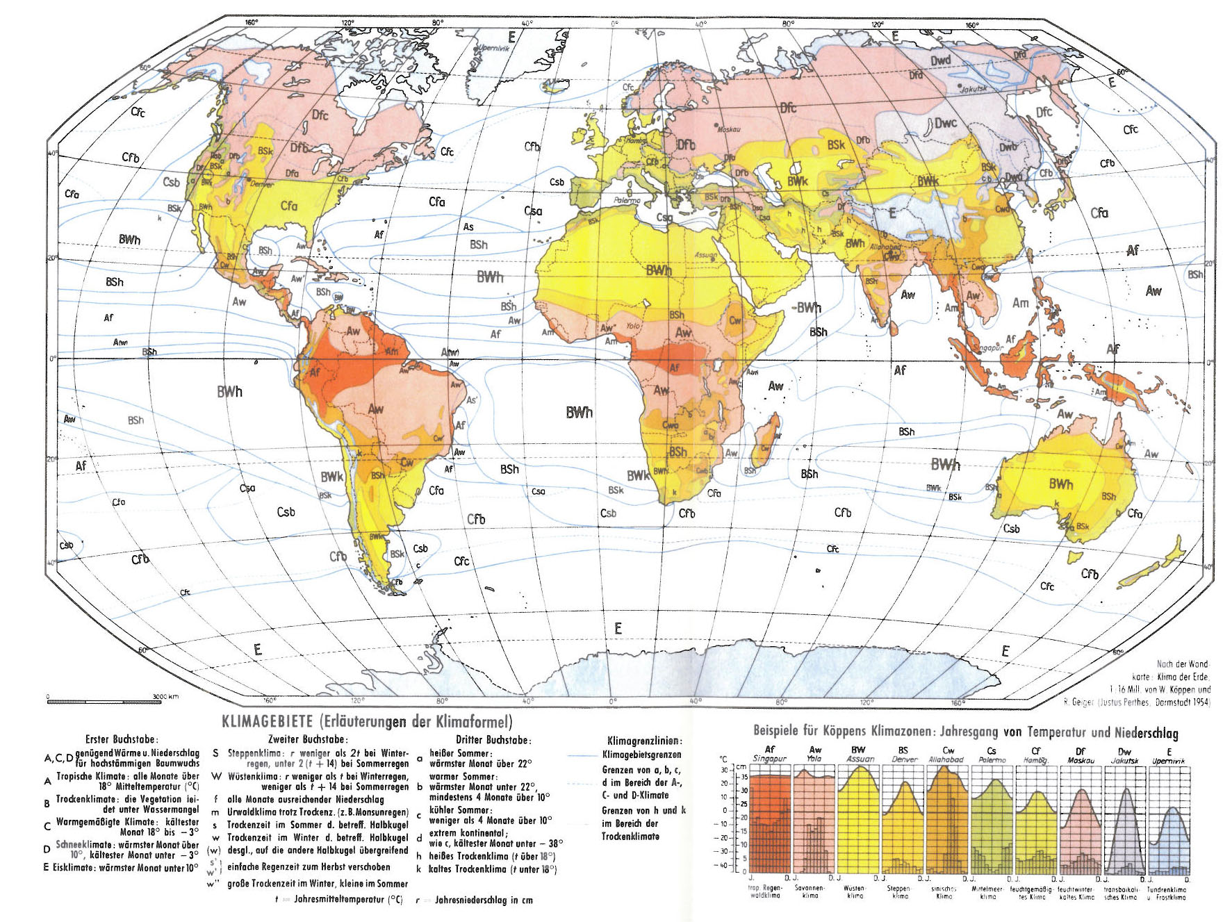
Cite this article
Yamanaka, M.D., Ogino, SY., Wu, PM. et al. Maritime continent coastlines controlling Earth’s climate. Prog Earth Planet Sci 5, 21 (2018). https://doi.org/10.1186/s40645-018-0174-9
Received:
Accepted:
Published:
DOI: https://doi.org/10.1186/s40645-018-0174-9