Drastic thickening of the barrier layer off the western coast of Sumatra due to the Madden-Julian oscillation passage during the Pre-Years of the Maritime Continent campaign

Abstract

The drastic thickening of the barrier layer in the marginal sea off the western coast of Sumatra during the passage of the Madden-Julian oscillation (MJO) observed during December 2015 is investigated. Before the MJO arrival, the halocline above a depth of 20 m was very strong, and the barrier layer thickness was 5–10 m based on R/V Mirai observations. During the MJO forcing of 13–16 December, the isothermal layer drastically deepened from 20 to 100 m. Meanwhile, the mixed layer deepening lagged behind the isothermal layer deepening by 1 day, and the barrier layer underwent dramatic thickening to 60 m within 24 h. An evaluation of the vertical salinity gradient tendency showed that the dramatic thickening of the barrier layer was due to the vertical oceanic mixing by the atmospheric MJO forcing and the vertical stretching by the oceanic downwelling coastal Kelvin wave intruding from the open ocean. In addition, an evaluation of the vertical temperature gradient tendency showed that the temperature inversion in the barrier layer formed by losing heat to the atmosphere due to the MJO forcing and downward advection of the temperature gradient due to the downwelling Kelvin wave resulting in the dramatic isothermal layer deepening. One of the important factors in the drastic barrier layer thickening was the atmospheric external forcing and the oceanic internal wave being in phase. The downwelling oceanic Kelvin wave continuously lowered the thermocline from the middle of November to the end of December, and the salinity stratification in the vicinity of the thermocline was continuously mitigated by the vertical stretching. Under such conditions, the MJO forcing caused vertical mixing of the freshwater with strong salinity stratification and temperature stratification near the surface. The combination of the two distinct processes caused the drastic thickening of the barrier layer, and the barrier layer thickness reached a maximum of 85 m 5 days after the MJO arrival.

Introduction

The layer between the top of the pycnocline and the top of the thermocline, the “barrier layer” (BL), is an ocean surface structure that plays a key role in the air-sea interaction processes (Anderson et al. 1996; Godfrey and Lindstrom 1989; Lukas and Lindstrom 1991; Sprintall and Tomczak 1992; Tomczak 1995). The BL forms a barrier to the entrainment and turbulent mixing of cold thermocline water into the mixed layer and inhibits the momentum of downward mixing (Vialard and Delecluse 1998a, 1998b). The formation mechanisms and seasonal variations of the BLs differ from region to region (Sato et al. 2004, 2006), and they are deeply involved in the Indian Ocean Dipole (IOD; Saji et al. 1999) (Masson et al. 2004; Qiu et al. 2012) and ENSO (Ando and McPhaden 1997; Maes et al. 2002, 2005; Maes et al. 2006). Previous studies have noted that the BL shows various responses to atmospheric forcing associated with westerly wind bursts and the continuous precipitation of the Madden-Julian oscillation (MJO; Madden and Julian 1971) (Cronin and McPhaden 2002; DeMott et al. 2015; Drushka et al. 2014).

Many previous studies of the BL over the open ocean have revealed that the horizontal advection, vertical tilting, and vertical stretching of the salinity stratification are primarily responsible for the formation of the BL. The thick BL over the western Pacific Ocean develops because of a strong downward circulation near the salinity front created by the convergence between the central Pacific salty water and fresher western Pacific water (Katsura et al. 2015; Vialard and Delecluse 1998a). A statistical analysis over the Pacific by Cronin and McPhaden (2002) revealed that the surface-intensified wind-driven jet tilts the zonal salinity gradient vertically when forming the BL during westerly wind bursts associated with the MJO.

Over the Indian Ocean, including the Bay of Bengal and Arabian Sea, the formation of the BL by the vertical stretching of the salinity stratification has been discussed in many previous studies (Girishkumar et al. 2011; Qiu et al. 2012; Thadathil et al. 2007; Thadathil et al. 2008). Qiu et al. (2012) noted that the BL seasonal variation was due to the IL variation regulated by the oceanic downwelling/upwelling Kelvin wave over the equatorial central Indian Ocean and off the western coast of Sumatra. Thadathil et al. (2007) and Girishkumar et al. (2011) showed that both downwelling by Rossby waves and Ekman pumping were effective for BL thickening in the Bay of Bengal, Arabian Sea, and in the vicinity of Sri Lanka. In addition to the vertical stretching effect, horizontal advection was discussed as a dominant factor in the BL formation mechanism (Masson et al. 2002; Masson et al. 2003).

Most previous studies on BLs are on open oceans, with few studies undertaken in coastal regions, including marginal seas and inland seas. Chu et al. (2002) showed the existence of a BL in the Sulu and Celebes seas (inland seas surrounded by the islands of Borneo and Mindanao) and suggested that the turbulent mixing of the surface freshwater is a major factor in BL formation. Zeng et al. (2009) also showed the existence of a BL in the southern and eastern basins of the South China Sea. However, such a vertical mixing process has not been directly validated by in situ high-frequency observations.

This study describes the drastic thickening of the BL during the MJO passage observed by the Research Vessel (R/V) Mirai cruise (MR15-04) as a part of a pilot campaign called “Pre-YMC” (Years of the Maritime Continent) in December 2015 (http://www.jamstec.go.jp/ymc/pre_ymc_2015.html). The R/V Mirai was stationed approximately 50 km off the western coast of Sumatra (4° S–102° E, 650~800 m bottom depth) in the shallow marginal sea of the Indian Ocean. A BL thickening from 5 to 60 m was observed 24 h after the MJO arrival, and the maximum BL thickness (BLT) was observed at 85 m depth 5 days after the MJO arrival. Such a drastic oceanic response to the MJO forcing was well documented by the high-frequency in situ observations of the R/V Mirai. The objective of this study is to reveal the daily scale drastic BLT increases associated with the MJO passage in the shallow marginal sea of the Indian Ocean. These in situ observations by the R/V Mirai are the first that capture the continuous BL variations in this area. Therefore, the results of this analysis using the R/V Mirai data as a case study are important for understanding the evolution of BL at a daily time scale. The data sources and definition of the BLT are presented in the “Data and definition of the BLT” section. The observed drastic BL thickening and BL formation processes are examined in the “Results and discussion” section. The conclusions are summarized in the “Conclusions” section.

Methods/Experimental

Data and definition of the BLT

The major component of the Pre-YMC campaign was the R/V Mirai (MR15-04 cruise), which was stationed approximately 50 km off the western coast of Bengkulu, Sumatra (4° S, 102° E, 650~800 m depth) from 23 November to 17 December in 2015 (Fig. 1; Yokoi et al. 2017; Wu et al. 2017). The basic surface meteorological observations (e.g., surface pressure, temperature, humidity, surface wind, precipitation, and sea surface temperature) were obtained every minute. Conductivity–temperature–depth (CTD) and lowered acoustic Doppler current profiler (LADCP) observations were conducted eight times per day, and the observed variables were interpolated over 2 m depth intervals. Microstructure measurements were made using a turbulence ocean microstructure acquisition profiler (TurboMAP) with a sampling rate of 512 Hz (Wolk et al. 2002) one to four times per day. The dissipation rates of the turbulent energy and temperature variance were computed by integrating the measured shear spectra and temperature variance over 5 m depth intervals, respectively.

Fig. 1

a Location of the observation sites and bathymetry (color, m). The red circle indicates the stationary observation site from 23 November to 17 December in 2015. The black circles indicate the 26 CTD observations from 00Z 21 November to 18Z 22 November at 10 km intervals. b The bathymetry along the line of A-A′ in (a). The maximum observation depth of the CTD observations is 500 m except for the locations at 00Z on 21 (1000 m), 17Z on 22 (374 m), and 18Z 22 (200 m) November. The periods between 00Z and 19Z on 21, 19Z on 21 and 06Z on 22, and 06Z and 18Z on 22 November correspond to the open Indian Ocean, oceanic ridge, and marginal sea, respectively

In addition to the fixed-point observations, an observation line along A-A′ (Fig. 1b) was conducted from 21 November to 22 November, and 26 CTD/LADCP profiles were obtained at approximately 20 km intervals. The observation line is bathymetrically divided into the open ocean (2000–6000 m), the oceanic ridge (800–2000 m), and the marginal sea (200–1500 m).

The BLT is defined as the difference between the isothermal depth (ILD) and the mixed layer depth (MLD) (de Boyer Montegut et al. 2004). The ILD is defined as the depth where the temperature is 0.2 °C lower than that at 10 m depth. Although this ILD definition includes both types of ILs with and without temperature inversion (Thadathil et al. 2007), the same definition is used throughout the profiles. The MLD is defined in terms of a depth with a density equal to that at the 10 m depth plus an increment in density equivalent to − 0.2 °C. This density increment is determined by the coefficient of thermal expansion, which is calculated as a function of the temperature and salinity. Therefore, the base of the mixed layer is the depth at which

$$ \uprho \mathrm{t},\mathrm{MLD}=\uprho \mathrm{t},10\mathrm{m}+\Delta \mathrm{T}\cdot \mathit{\partial \rho }/\mathrm{\partial T}, $$

(1)

where ρ_t,10m is the density at 10 m depth, ΔT is 0.2 °C and ∂ρ/∂T is the coefficient of thermal expansion.

The Estimating the Circulation and Climate of the Ocean, Phase II (ECCO2) cube92 dataset has 50 vertical levels ranging in thickness from 10 m near the surface to approximately 450 m at a maximum model depth of 6150 m with a high-resolution global ocean 0.25° × 0.25° (Halpern et al. 2015; Menemenlis et al. 2008). The ECCO2 is an adjoint method state estimate constrained to the available satellite (sea surface temperature and height) and in situ (vertical temperature and salinity profiles) data.

A globally merged infrared radiation brightness temperature (Tb) dataset was used to depict the evolution of the MJO convection (Janowiak et al. 2001). The Japanese 55-year reanalysis JRA55 (Ebita et al. 2011; Kobayashi et al. 2015) was used to capture the westerly winds associated with the MJO.

Results and discussion

Observed BL evolution during the MJO passage

Figure 2 shows the time-depth sections of the CTD and LADCP observations along the A-A′ line in Fig. 1. The ocean surface structure in the marginal sea (06-18Z on 22 November) was significantly different from that in the open ocean (00-18Z on 21 November). In the marginal sea, the temperature was 1 °C higher, and the salinity was 1 psu (practical salinity unit) lower than those in the open ocean 0–20 m layer. The vertical gradients of the density (Fig. 2a), temperature (Fig. 2b), and salinity (Fig. 2c) in the 6–10 m layer are indicated by the bars at the top of each panel as a surface stratification index. The purple bars indicate that the vertical gradient in the 6–10 m layer was small (less than 0.01 kg/m⁴, 0.03 °C/m, and 0.013 1/m) and that the surface layer above the reference depth of 10 m was sufficiently vertically mixed. The thresholds of 0.03 °C/m and 0.013 1/m are approximately equivalent to the density gradient of 0.01 kg/m⁴ under the condition that the temperature and salinity are 30 °C and 32 psu, respectively. We introduced the indices to distinguish the different regimes with and without the strong surface stratification above the reference depth of 10 m. The surface density stratification index exceeding 0.01 kg/m⁴ was confined in the marginal sea. The depth of the local maximum of the fluorescence and dissolved oxygen distributions were also clearly different between the marginal sea and the open ocean. In addition, the horizontal current speed in the marginal sea was very low (5–35 cm/s). This result suggests that the horizontal advection effect on the formation of the BL in the marginal sea is less than that in the open ocean.

Fig. 2

Time-depth sections of a the density, b the potential temperature, c the salinity, d the fluorescence (relative units), e dissolved oxygen (umol/kg), and f the horizontal current velocity along the A-A′ line in Fig. 1. The dashed and dotted lines indicate the MLD and ILD, respectively. The blue line indicates the 29, 25, and 20 °C isotherms. The surface wind speed is superimposed in f with the right axis. The 2-hour running mean is adopted for each variable. The periods of the open Indian Ocean, oceanic ridge, and marginal sea defined by the bathymetry in Fig. 1 are indicated at the bottom in each panel. The bars at the top of each panel show the vertical gradients of the density, temperature, and salinity between 6 and 10 m (green: values more than 0.01 kg/m⁴, 0.03 °C/m, and 0.013 1/m, purple: less than 0.01 kg/m⁴, 0.03 °C/m, and 0.013 1/m)

Figure 3 shows the time-longitude cross section of the Tb and the surface westerly wind speed averaged for 5° S–5° N. The large-scale cloud system associated with westerly winds passed over the R/V Mirai after 11 December (Wu et al. 2017; Yokoi et al. 2017). This MJO was in phase 4 (the western part of the Maritime Continent) during 7–16 December and phase 5 (the western part of the Maritime Continent) during 17–22 December by the Bureau of Meteorology’s MJO index (Wheeler and Hendon 2004).

Fig. 3

Time-longitude cross-section of the Tb (color, K), the surface westerly wind speed (blue contours for every 1 m/s) averaged for 5° S–5° N from 20 November to 31 December in 2015. The bold red dashed line indicates the location of R/V Mirai from 23 November to 17 December in 2015

Figure 4 shows the time series of the 24-hour running mean of the MLD, ILD, BLT, and surface wind speeds. The MLD (black) was deepening up to 45 m during the MJO passage for 13–17 December, even though it was less than 15 m, and it barely responded to the wind speed variation before 13 December. Meanwhile, the ILD (blue) was monotonically deepening up to 110 m during the MJO, which was associated with two peaks of the surface wind speed greater than 8 m/s.

Fig. 4

Time series of the 24-hour running mean MLD (black), ILD (blue), BLT (red), and surface wind speed (black dashed) at the stationary site of the R/V Mirai

As a result, the BLT (red) variation shows distinct features before and after the MJO passage. Before 13 December, the BLT was less than 10 m during the period with a calm condition (< 3 m/s), and the BL thickened to approximately 25 m after a moderate wind peak of 3–6 m/s (27–30 November and 4–7 December). The time delay (2–3 days) of the BL thickening from the wind peak could depend on the strength of the surface stratification shown in Fig. 5. On 13 December, the BL drastically thickened to 60 m within 24 h, corresponding to the strong wind peak exceeding 9 m/s. On 15–16 December, the BLT thinned to 45 m because of the ML deepening associated with the second peak of the surface wind speed exceeding 8 m/s. On 16–17 December, however, the MLD shallowed again, resulting in the BL thickening up to 85 m. This value is very large compared with those found in previous statistical studies (Drushka et al. 2014; Sato et al. 2004, 2006; Vissa et al. 2013a).

Fig. 5

Time-depth sections of a the density, b potential temperature, c salinity, d fluorescence (relative units), e horizontal current velocity, and f dissipation rate of the turbulent kinetic energy at the stationary site of the R/V Mirai. The dashed and dotted lines indicate the MLD and ILD, respectively. The blue line indicates the 29 °C isotherm. The surface wind speed is superimposed in e and f with the right axis. The 24-hour running mean is adopted for each variable except for the dissipation rate of the turbulent kinetic energy. The bars at the top of each panel show the vertical gradients of the density, temperature, and salinity between 6 and 10 m (green: values more than 0.01 kg/m⁴, 0.03 °C/m, and 0.013 1/m, purple: less than 0.01 kg/m⁴, 0.03 °C/m, and 0.013 1/m)

Before the MJO passage, there were two events of BL thickening up to 20–25 m in the periods of 27–30 November and 4–7 December. For these two events, the preceding peaks of the surface wind (3–6 m/s) speed were weaker than the wind speeds during the MJO passage. Additionally, the BL is hardly thickened on 7 December, despite a relatively strong wind of 5 m/s. Therefore, the BL thickening (40–85 m) associated with the MJO passage was clearly distinct from the BL variations before the MJO passage.

Figure 5 shows time-depth sections of the CTD, LADCP, and TurboMAP observations. Before the MJO arrival on 13 December, the density in the layer of 4–10 m depth was very small (< 20 kg/m³), and the density stratification was significant (Fig. 5a). This low-density surface layer was due to the high temperature (> 29.5 °C; Fig. 5b) and low salinity (< 32.5, Fig. 5c) and could be freshened by the continuous precipitation off the western coast of Sumatra. In particular, the vertical gradients of the density (Fig. 5a) and salinity (Fig. 5c) between 6 and 10 m (the surface stratification indices shown by the bars at the top of each panel) exceeded 0.1 kg/m⁴ and 0.2 1/m during 6–12 December. Such significant surface salinity stratification above the reference depth of 10 m is a potential source of salinity stratification below 10 m by vertical mixing and downward advection (Fig. 5c). After the MJO arrival, the surface density stratification index rapidly decreased, and the stratification in the 10–60 m layer mitigated on 13 December, while the pycnocline decreased below 60 m after 14 December (Fig. 5a).

The temperature at approximately 10 m depth was continuously higher than 29.5 °C after 1 December and reached up to 30 °C, resulting in a surface temperature stratification index (6–10 m depth) greater than 0.03 °C/m on 12 December just before the MJO arrived (Fig. 5b). The IL was drastically deepened just after the MJO arrived on 13 December, and the temperature inversion in the BL (Balaguru et al. 2012; Cronin and McPhaden 2002; Mignot et al. 2012; Thadathil et al. 2002; Vinayachandran et al. 2002; Vissa et al. 2013b) is significant during the MJO passage. Meanwhile, the contour of the 29 °C contour, which is indicative of the top of the thermocline, was continuously sinking throughout the observation period.

Although the salinity in the 4–10 m layer was continuously less than 32.5 after 27 November, the salinity in the ML during the period of 14–16 December increased to 32.7 (Fig. 5c). On 13 December, the strong stratification with low salinity, i.e., less than 32.5 in the 4–10 m layer and the ML deepening, showed a 1-day lag with the IL deepening. The 1-day lag could be from the time scale due to the process that the strong surface stratification with the low salinity in the 4–10 m layer was vertically well mixed in, and the surface density stratification index became 0.01 kg/m⁴ or less.

The peak of phytoplankton fluorescence concentration (Fig. 5d) continuously shifted from 20–80 m to 50–110 m due to thermocline sinking throughout the observation period. During the MJO passage, relatively large values greater than 0.2 (relative units) were distributed in the 4–100 m layer, suggesting the occurrence of strong vertical mixing.

The variation in the horizontal current speed (Fig. 5e) could be due to its acceleration with the wind stress and diurnal luni-solar tide (here, the variation with the semidiurnal tide was smoothed by a 24-hour running mean). Before the MJO arrival, the current speeds were basically very slow (2–20 cm/s), although some speeds exceeding 20 cm/s were observed during the spring tide (26–27 November) and neap tide (8–9 December); that is, the contribution of the horizontal advection term that is significant in the formation of the BL over the open ocean could be quite small. In fact, the current speed on 13 December when the BL drastically thickened was less than 10 cm/s. Meanwhile, current speeds greater than 20 cm/s in the ML after 14 December corresponded to the wind speed peak with a 1-day delay.

Prior to the MJO arrival, in the layer below 30 m, the log₁₀(ε) values (Fig. 5f) before the neap tide (9 December) were relatively large (− 9~− 7), and those during the period between the neap tide and MJO arrival (8–12 December) were small (− 11~− 9). In the 10–30 m surface layer, the variation in log₁₀(ε) corresponded well to that of the surface wind speed and suggested vertical mixing associated with wind stress variations. After the arrival of the MJO, significant increases in log₁₀(ε) corresponding to the surface wind speed peaks were observed on 13 and 15 December. This result suggests that vertical mixing strongly contributed to drastic BL thickening, although the significant increases in log₁₀(ε) did not sufficiently reach the bottom of the IL.

Figure 6 shows the vertical profiles of the daily averaged density, salinity, and temperature for 12–17 December. On 12 December (Fig. 6a), the salinity and temperature stratifications were very strong in the 4–20 m layer (1 per 10 m = 0.1 1/m and 0.5 °C per 10 m = 0.05 °C/m). Additionally, there was a moderate salinity stratification in the 20–70 m layer (0.5 per 50 m = 0.01 1/m), which was a potentially favorable condition for thick BL formation. Additionally, a strong temperature stratification was observed only near the surface, and the temperature in the 20–40 m layer was well mixed at approximately 29.6 °C. Such a temperature profile could be a potentially favorable condition for drastic IL deepening. On 13 December (Fig. 6b), a strong wind peak exceeding 9 m/s was observed as the first MJO forcing. The salinity stratification in the 4–20 m layer was mitigated by a vertical gradient of 0.1 1/m to 0.02 1/m, and the temperature of approximately 29.6 °C was vertically well mixed in the 4–40 m layer above the top of the temperature inversion. Although the vertical salinity gradient in the 4–70 m layer was mitigated to approximately 0.02 1/m, the ML was not deepened because of the strong density stratification (0.01–0.05 kg/m⁴; Fig. 6a) associated with the salinity stratification (0.1–0.5 1/m; Fig. 6b) remained in the surface layer above the reference depth of 10 m. As a result, the BL was drastically thickened to approximately 60 m within 1 day. On 14 December (Fig. 6c), the ML deepened to 30 m after the mitigation of the salinity stratification. In contrast, the IL slightly deepened by a few meters per day due to a sinking thermocline, and the BL was thinned back to 40 m. The temperature inversion that is a BL feature appeared in the 50–70 m layer.

Fig. 6

Vertical profiles of the density (black), salinity (blue, top axis), and temperature (red, bottom axis) averaged for a 12, b 13, c 14, d 15, e 16, and f 17 December in 2015 at the stationary site of the R/V Mirai. The solid and dashed lines indicate the MLD and ILD, respectively

On 15 December (Fig. 6d), a strong wind peak exceeding 8 m/s was observed as the second MJO forcing. The salinity stratification in the layer of 4–60 m was further mitigated, and the ML deepened to 40 m. Meanwhile, the deepening of the IL slowly continued (5–10 m per day), and the BLT remained at approximately 40 m. On 16–17 December (Fig. 6e, f), the IL deepening slowly continued, and the 4–20 m layer freshened in association with the MJO precipitation. This freshening could be due to the large P − E exceeding 130 mm over 2 days, which was associated with the continuous precipitation following the decreased evaporation from the weakened wind speed. The salinity decrease of approximately 0.1 per day in the 0–20 m layer is consistent with the calculation based on S′ = S(P − E)/h (S = 32.5, P − E = 65 mm/day, h = 20 m, and S′ ≒ 0.1). Because the MLD became shallow, i.e., less than 20 m, due to the freshwater flux from the MJO precipitation and the IL continuously deepened to 100 m, the BL thickened again to the maximum of 85 m.

Evaluation of the vertical salinity gradient balance

Figure 7 shows the time-depth sections of the variables related to the vertical salinity gradient tendency. Although the quantitative analysis of each following term is difficult from the fixed observation locations, the formation of the BL can be partly inferred from the qualitative tendency. According to Cronin and McPhaden (2002), the vertical derivative of the salinity balance equation to estimate the surface salinity stratification is

Fig. 7

Time-depth sections of a the tendency of the vertical salinity gradient (× 10⁻¹ 1/m/day), b the vertical salinity gradient (× 10⁻¹ 1/m), c the second-order derivative of salinity (× 10⁻² 1/m²/day), d the tendency of the salinity (× 10⁻¹ 1/day), e the vertical gradient of the zonal velocity (× 10³ 1/day), f the dissipation rate tendency of the turbulent kinetic energy (W/kg/day) at the stationary site of the R/V Mirai. The blue line indicates the 29 °C isotherm. The dashed and dotted lines indicate the MLD and ILD, respectively. The surface wind speed (m/s) is superimposed in f with the right axis. The black bars at the top of a–d show freshwater flux (×10⁻¹ m/day)

where U is the horizontal velocity, ω is the vertical velocity, ∇ is the horizontal gradient operator, and $\overline{\omega^{\prime }S^{\prime }}$ is the vertical turbulent salinity flux. The vertical turbulent salinity flux at the sea surface depends on the surface salinity (S₀, 32~32.5) and the freshwater flux from the precipitation minus the evaporation (P – E, − 0.01~0.1 m/day) according to

$$ \overline{\left({\omega}^{\prime }{S}^{\prime}\right)}\left|{}_{z=0}\right.={S}_0\left(P-E\right). $$

(3)

This condition applies to the turbulent vertical mixing component (term 5) of (2) at the surface, and its order is approximately 10⁰–10⁻² m/day. It is expected that the order of the term 5, $-\overline{{\left({\omega}^{\prime }{S}^{\prime}\right)}_{zz}}$, is 10⁻²–10⁻⁴ m/day, assuming an order reduction by taking the second-order differential as 10⁻².

Thus, the formation and growth of the BL are evaluated by the vertical salinity gradient tendency Eq. (2), which contains the horizontal advection (term 1), the vertical advection (term 2), the tilting of a horizontal salinity gradient by a vertical sheared horizontal flow (term 3), the vertical stretching of the vertical salinity gradient (term 4), and the vertical turbulent salinity flux originating from the surface freshwater (term 5).

As shown in Fig. 7a, the order of S_zt was 10⁻¹–10⁻² m/day. The increase in S_zt near the surface corresponds to that of the freshwater flux for the periods of 24 November, 6–8 December, and 11 December, indicating the large surface stratification indices (greater than 0.2 kg/m⁴ and 0.2 1/m) and a very shallow IL less than 20 m in depth. The very shallow IL could be due to the surface stratification because the incoming heat could be used for shallow ML warming. In contrast, three pairs of positive and negative S_zt values around the bottom part of IL and in the middle of IL declined with time for the periods of 27–30 November, 3–6 December, and 13–17 December, indicating a small surface density stratification index and an IL deepening more than 20 m depth. These pairs of positive and negative S_zt values in the IL correspond well to the increased turbulence kinetic energy dissipation rate shown in Fig. 7f. This result suggests that vertical mixing induces salinity stratification reduction near the surface and intensification around the bottom part of the IL. Thus, Fig. 7a, f suggest that term 5 in Eq. (2) was important for the drastic thickening of the BL on 13 December. Additionally, the S_t in the BL (Fig. 7d) was continuously negative for 13–16 December, which supports the notion that the lower salinity near the surface was vertically mixing into the BL. In fact, the ML also deepened for 13–16 December by the relaxation of the surface salinity stratification, as shown in Fig. 6b–e.

As for S_z in Fig. 7b, a very strong salinity stratification near the surface before 12 December was stretched in the 20–70 m layer on 13 December. This S_z distribution suggests that term 4 in Eq. (2) of the vertical stretching was also effective. In addition, the large positive S _z (> 1 × 10⁻¹/m) indicated by the warmer colors was seen around the bottom part of the IL for 14–17 December, and the positive S_zt around the bottom part of the IL is considered to be generated by the vertical stretching associated with the continuous sinking thermocline under ω _z  < 0, which is supported by the ECCO2, as in Fig. 9d. Term 4 of − ω_zS_z would contribute to the positive S _zt , and its order could be approximately 10⁻²–10 ³ m/day, assuming ω _z to be 10⁻¹–10⁻² 1/day.

Concerning the S_zz distribution related to the vertical advection (Fig. 7v), the positive and negative S_zz pair in the sinking thermocline (around the 29 °C isotherm) was observed throughout the observation period. If the vertical motion was negative (ω < 0), the vertical advection term partly contributed to the positive S_zt around the bottom part of the IL. Term 2 of − ωS _zz would be positive, and its order could be approximately 10⁻²–10⁻³ m/day, assuming the order of ω to be 10⁰–10⁻¹ 1/day.

The vertical shear of the zonal current (Fig. 7e) is related to term 3 of the tilting effect. The speculated horizontal gradient of the salinity would be negative because the higher and lower salinity values could be to the west and east, respectively. The speculated order of ∇S from Fig. 2c could be approximately 10⁻⁵–10⁻⁶/m, and the order of term 3 could be approximately 10⁻²–10⁻³/m/day. The vertical shear in the BL for 13–16 December was generally negative, and the tilting term could not be effective for BL formation. In fact, the vertical shear variation was not generally correlated with the S_zt variation, and the negative S_zt corresponds to the minimum vertical shear just under the deepening ML on 14 December. The order of the vertical shear of the meridional current was 10² 1/day (not shown), and the meridional component of the tilting effect must be even smaller than the zonal component.

Considering the zonal component of term 1, its order could be approximately 10⁻³–10⁻⁴/m/day based on the small zonal current speed of less than 10 cm/s (~ 10³ m/day; see Fig. 5e), assuming ∇S_z to be 10⁻⁶~10⁻⁷/m² based on Fig. 2c. The meridional component of term 1 could be even smaller because of the smaller meridional current speed than the zonal one. In addition, the current speed distribution was not consistent with the pair of positive and negative S_zt in the BL. Thus, the advection term could not be as dominant for BL formation compared with the previous studies in open oceans (e.g., Cronin and McPhaden 2002). Note that the horizontal advection due to the current direction variation and surrounding fresh lens is speculated to be effective for the higher frequency variation (less than 24 h) of the surface salinity, although it is beyond the scope of our study due to the smoothing by the 24-hour running mean.

Evaluation of the vertical temperature gradient balance

Figure 8 shows the time-depth sections of the variables related to the vertical potential temperature gradient tendency. Often, the vertical gradient tendency of the temperature is correlated with that of the salinity. According to Cronin and McPhaden (2002), the vertical derivative of the temperature balance equation to estimate the surface temperature stratification is

Fig. 8

Time-depth sections of a the tendency of the vertical temperature gradient (°C/m/day), b the second-order derivative of temperature (× 10⁻² °C/m²), c the tendency of the temperature (°C/day), d the vertical gradient of the potential temperature (°C/m), and e the dissipation rate of the temperature variance (°C²/s) at the stationary site of the R/V Mirai. The blue line indicates the 29 °C isotherm. The dashed and dotted lines indicate the MLD and ILD, respectively. The black contours of 29, 25, 20, and 15 °C are shown in d and e

where ρcp is the volumetric heat capacity, Qrad is the penetrative solar radiation, and $\overline{\omega^{\prime }T^{\prime }}$ at z = 0 is proportional to the net surface heat flux reduced by the solar radiation at the surface. Although it was difficult to directly estimate terms 5 and 6, the net surface heat flux was confirmed to become negative (~− 1 °C/day for 50 m depth: negative means losing heat to the atmosphere) during the MJO wind burst forcing from the surface meteorological observation (not shown) and daily averaged temperature near the surface was decreased, as shown in Fig. 6. This result suggests that terms 5 and 6 contribute to the vertical potential temperature gradient tendency and is consistent with the development of the temperature inversion in the layer of 40–80 m depth. As shown in the profiles of Fig. 6a, b, the decreased temperature stratification near the surface led drastic IL deepening. Additionally, the temperature in the 20–50 m depth layer on 12 December (Fig. 6a) was mixed at approximately 29.6 °C, and such conditions were potentially favorable for drastic IL deepening. That is, before the IL deepening, there was a potential condition of the mixed temperature just below the surface halocline, and the temperature stratification existed only near the surface above 20 m depth. After losing heat to the atmosphere near the surface, the temperature stratification near the surface disappeared, and the ILD value drastically increased. However, because the salinity stratification in the IL remained, the ML deepening showed a 1-day lag with the IL deepening.

The vertical potential temperature gradient tendency basically supports the estimation in the salinity balance in the previous section. As shown in Fig. 8a, the order of T_zt was 10⁻² °C/m/day in the IL. The positive T_zt values in the IL on 13 December suggest decreased temperature stratification by vertical mixing. In fact, the contribution of the horizontal advection of term 1 could be small because its order could be approximately 10⁻³–10⁻⁴ °C/m/day based on the small current speed of less than 10 cm/s (~ 10³ m/day; see Fig. 5e), assuming ∇T_z to be 10⁻⁶~ 10⁻⁷ °C/m² based on Fig. 2b. In contrast, as shown in Fig. 8b, term 2 of −ωT _zz would be positive in the upper BL and negative in the lower BL under ω < 0 (see Fig. 9d). Its order could be approximately 10⁻²–10⁻³ °C/m/day, assuming the order of ω to be 10⁰–10⁻¹ 1/day, suggesting that the downward advection of the temperature inversion from the upper BL to the lower BL occurs and that it is possible to develop the temperature inversion when strong winds lose heat near the surface to the atmosphere. Additionally, negative T_t values from the surface in the IL (Fig. 8c) were continuously shown after 13 December, which supports the notion that the temperature in the upper IL was decreased by the losing heat to the atmosphere and vertical mixing. For the tilting effect of term 3, the speculated order of ∇T from Fig. 2b could be approximately 10⁻⁵–10⁻⁶ °C/m, and the order of term 3 could be approximately 10⁻²–10⁻³ °C/m/day.

Fig. 9

Time-depth sections of a the potential temperature (°C), b the salinity, c the current speed (cm/s), and d the vertical motion (× 10³ cm/s) at the grid of 4.375° S, 101.875° E with ECCO2. The dashed and dotted lines indicate the MLD and ILD, respectively. The surface wind speed with JRA55 and the SSH with ECCO2 are superimposed in c and d with the right axis

As for T _z in Fig. 8d, the positive T _z (1 × 10⁻¹–10⁻² °C/m) indicated by the warmer colors was sinking in the middle of the BL during the MJO passage. This sinking positive T _z means that the upper part of the temperature inversion is sinking in the middle of BL. The positive T _zt in the middle of the BL in Fig. 8a is considered to be generated by the vertical stretching under ω _z  < 0, which is supported by the ECCO2 as in Fig. 9d. Term 4 of − ω _z T _z would contribute to the positive T _zt , and its order could be approximately 10⁻²–10⁻³ °C/m/day, assuming ω _z to be 10⁻¹–10⁻² 1/day.

The local minima of the vertical gradient of the potential temperature were observed in the 50–200 m layer along the 29, 25, 20, and 15 °C isotherms. The positive vertical gradients (Fig. 8d) in the surface layer (4–20 m) often appeared in association with the SST decrease (27–28 November, 30 November, 4–5 December, and 8–10 December). After the arrival of the MJO, the local maxima of the positive vertical gradients indicated the temperature inversion feature in the BL. The large dissipation rate of the temperature variance in the 50–200 m layer (Fig. 8e) corresponded well to the minima of the vertical gradients of the potential temperature. The layer with the large dissipation rate of the temperature variance was sinking significantly over 1–17 December, suggesting a downwelling associated with a large-scale oceanic wave.

Role of the downwelling coastal oceanic Kelvin wave

Figure 9 shows the time-depth sections at the grid nearest to the R/V Mirai from ECCO2 (4.375 S, 101.875 E). ECCO2 has a high-temperature bias of 0.3–0.4 °C in the surface layer throughout the observation period (Fig. 9a). Although the continuous sinking of the thermocline in ECCO2 is consistent with the observation, the observed drastic IL deepening on 13 December was not well represented. This observation was because the 10 m vertical resolution was too coarse to represent the observed strong stratification near the surface before the MJO arrival. Meanwhile, the ILD and MLD variations with a reference depth of 20 m depth were consistent between the observation and ECCO2, and the ECCO2 well represents the observed structure below 20 m depth. In fact, the temperature inversion was also represented after 13 December, as shown in Fig. 5b. The salinity from ECCO2 (Fig. 9b) was generally underestimated by 0.2–0.7 compared with the observation. However, the surface salinity reached the minimum on 9 December, and the salinity in the IL was vertically well mixed for 13–17 December, which is consistent with the observations.

Although the horizontal current speed in ECCO2 (Fig. 9c) was slightly overestimated compared with the observation, the accelerated current during the MJO passage was well represented. The intensification of the surface wind speed from JRA55 was slightly underestimated by 3–5 m/s compared with the observation. Because the observed two peaks associated with the MJO are represented, the MJO’s influence is included in the atmospheric forcing in ECCO2 that adopts the JRA55 dataset as the surface condition. Although the vertical velocity (Fig. 9d) cannot be validated because of the inadequate technology of directly measuring the vertical velocity in a real ocean, the downwelling is obviously dominant associated with the continuous increase in the sea surface height during the observation period. This result is consistent with the observed continuously sinking thermocline. ECCO2 represents the observed variations in temperature, salinity, and horizontal current, although it includes biases. Thus, the fact that downwelling is dominant in ECCO2 is sufficiently reliable.

Figure 10 shows the horizontal distributions of the sea surface height (SSH), SST, vertical motion, isotherm depth of 20 °C, salinity, and BLT averaged between 23 November and 17 December. Over the Indian Ocean, the SSH to the east is generally higher than that to the west (Fig. 10a). The SSH distribution is consistent with the surface wind distribution in which the westerlies are dominant over the equator. The highest SST over the Indian Ocean (Fig. 10b) is shown off the west coast of Sumatra corresponding to the higher SSH. The large-scale downwelling over the equator and along the western coast of Sumatra (Fig. 10c) is associated with the westerly currents and suggests the presence of an oceanic equatorial and coastal Kelvin wave that is excited by the westerly winds. The 20 °C isotherm depth over the equator is more than 100 m, suggesting that the thermocline is deepened by the oceanic downwelling equatorial/coastal oceanic Kelvin wave (Fig. 10d). The eastward current near the surface (45–155 m) is dominant over the equator, and the low salinity area is confined near the coast to the west of Sumatra (Fig. 10e).

Fig. 10

Averaged horizontal distribution of a SSH (cm), b SST (°C), c the vertical motion averaged between 45 and 155 m (× 10³ cm/s), d the depth of the 20 °C isotherm (m), e the salinity averaged between 45 and 155 m, and f the BLT (m). The surface wind vectors with JRA55 are shown in a and b. The ocean current vectors averaged between 45 and 155 m with ECCO2 are shown in c–e. The sections in Fig. 11 are plotted along the black solid line

The thick BLT of more than 20 m was distributed in the areas over the equatorial central Indian Ocean, off the western coast of Sumatra, in the Bay of Bengal, and in the vicinity of Sri Lanka (Fig. 10f). This thick BL distribution is consistent with previous studies describing the BL formation in the areas over the equatorial central Indian Ocean and off the western coast of Sumatra (downwelling oceanic Kelvin wave; Qiu et al. 2012), in the Bay of Bengal (the downwelling by the oceanic Rossby wave and related Ekman pumping; Thadathil et al. 2007), and in the vicinity of Sri Lanka (the downwelling oceanic Rossby wave; Girishkumar et al. 2011).

Figure 11 shows the time-longitude cross sections of sea level anomalies (SLA) from the temporal average for the period of 1 October–31 December, SST, vertical velocity averaged between 45 and 155 m depths, isotherm depth of 20 °C, salinity averaged between 45 and 155 m depths, and the BLT from ECCO2. These are the sections along the black solid line in Fig. 10 for extracting the equatorial and coastal Kelvin wave. Between the middle of October and the end of December, the westerly winds gradually expanded eastward from the western Indian Ocean, and the eastward propagation of the positive SLA (the phase speed of approximately 1 m/s) was observed (Fig. 11a). The eastward propagation of the higher SST was more than 29.5 °C (Fig. 11b), and the descending velocity (Fig. 11c) and the 20 °C isotherm depth corresponded well with that of the positive SLA (Fig. 11d). The BLT showed an eastward propagating signal from the central to the eastern Indian Ocean for the 2 months of November and December (Fig. 11f), which corresponded well with the eastward propagation of the negative salinity anomaly in the surface layer (Fig. 11e); that is, the downwelling Kelvin wave excited by the westerly winds over the western Indian Ocean in mid-October reached the west coast of Sumatra Island in December. The continuously sinking thermocline observed at the R/V Mirai could be due to the downwelling coastal oceanic Kelvin wave from late November to the middle of December. The fact that the MJO and oceanic downwelling Kelvin wave were in phase could be important for drastic BL thickening.

Fig. 11

Time-depth sections of a SLA (cm), b SST, c the vertical motion averaged between 45 and 155 m (× 10³ cm/s), d the depth of the 20 °C isotherm (m), e the salinity anomaly from the temporal mean for October–December averaged between 45 and 155 m, and (f) BLT (m) with ECCO2. The surface westerly wind speed (blue contours for every 1 m/s) is shown in a and b. The ILD (white contours for every 10 m) is shown in f. The bold black line in each panel indicates the fixed observation period of R/V Mirai

Conclusions

This study reveals a drastic thickening of the BL off the western coast of Sumatra (4° S–102° E, 600~800 m bottom depth) during the MJO passage observed during December 2015. The BL formation process is explained on the basis of the vertical salinity gradient balance equation using unique R/V Mirai (MR15-04 cruise) in situ observations collected during the Pre-YMC campaign. ECCO2 supported the analysis of the BL formation process.

Figure 12 is a conceptual diagram depicting the change in characteristics of the temperature-salinity profile characteristics with respect to the drastic BL thickening. There are two strong atmospheric forcing events accompanying the MJO at the R/V Mirai, and the BL development process can be divided into the following 6 forcing-based stages.

• Stage 1: Just before the first wind burst (WB) forcing (the daily averaged surface wind speed of approximately 6 m/s and the daily freshwater flux of 36 mm/day) on 12 December

• Stage 2: The first WB peak (9 m/s, 5 mm/day) on 13 December

• Stage 3: The first weakened WB forcing/just before the second WB forcing peak (6 m/s, 10 mm/day) on 14 December

• Stage 4: The second WB forcing (9 m/s, 74 mm/day) on 15 December

• Stage 5: The second weakened WB forcing (6 m/s, 61 mm/day) on 16 December

• Stage 6: After the second WB forcing (3 m/s, − 1 mm/day) on 17 December

  Fig. 12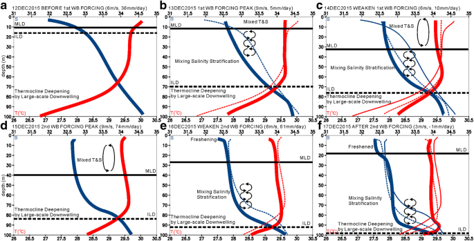

  

  Schematic profiles of the salinity (blue, top axis) and temperature (red, bottom axis) a before the 1st wind burst (WB) forcing on 12 December (6 m/s, 36 mm/day), b during the 1st WB forcing peak on 13 December (9 m/s, 5 mm/day), c during the 1st weakened WB forcing on 14 December (6 m/s, 10 mm/day), d during the 2nd WB forcing on 15 December (9 m/s, 74 mm/day), e during the 2nd weakened WB forcing on 16 December (6 m/s, 61 mm/day), f after the 2nd WB forcing on 17 December (3 m/s, − 1 mm/day) in 2015. The solid and dashed lines indicate the MLD and ILD, respectively

At stage 1 (Fig. 12a), the 0–20 m surface layer was associated with extremely strong salinity (0.1/m²) and temperature stratification (0.05 °C/m²), and the MLD and ILD were extremely thin because there was a density stratification between the surface and the reference depth of 10 m. We introduced indices for the surface stratification defined by the vertical gradients of the density, temperature, and salinity between 6 and 10 m to distinguish the different regimes with and without the strong surface stratification above the reference depth. The surface salinity stratification index at stage 1 was more than 0.1/m⁴. In addition, there was a moderate salinity stratification (0.01/m) in the 20–70 m layer that was a potential condition for forming a thick BL. Additionally, a strong temperature stratification was observed only near the surface above 20 m, and the temperature in the 20–40 m layer was well mixed. Such a temperature profile could be a potentially favorable condition for drastic IL deepening.

At stage 2 (Fig. 12b), due to the first WB forcing, the strong salinity stratification in the surface layer was mitigated, and the temperature stratification was dissolved, resulting in a surface salinity stratification index at stage 2 less than 0.01/m⁴. The IL drastically deepened to a depth of 70 m within 24 h. However, moderate salinity stratification (a 0.02/m vertical salinity gradient) remained in the 0–70 m layer, and the ML was not deepened so that the BL thickened dramatically up to 60 m.

At stage 3 (Fig. 12c), as the first WB forcing weakened, the salinity was well mixed in the 0–40 m layer, and the ML deepened to 30 m. On the other hand, the IL continued to slowly deepen at 5–10 m/day associated with the descending of the thermocline due to the coastal downwelling oceanic Kelvin wave. The BL thinned to 40 m because of the ML deepening. At this stage, in the 50–70 m layer, a temperature inversion, which is a BL feature, remarkably appeared because of the loss of heat from the ML to the atmosphere and downward advection of higher temperature at approximately 29.6 °C in the lower IL.

At stage 4 (Fig. 12d), under the second WB forcing, the salinity stratification of the surface layer was further mitigated, and the ML deepened to 40 m depth. In contrast, the IL continued to slowly deepen at approximately 5–10 m/day, and the BLT remained at 40 m.

At stage 5 (Fig. 12e), as the second WB forcing weakened, the salinity stratification strengthened again in the surface of the 0–20 m layer. The surface salinity stratification of an approximately 0.1 salinity decrease was due to continuous precipitation (P) by the MJO resulting in a larger P − E (74 mm/day on 15 December at stage 4). The BL began to thicken again because the MLD became shallow despite continuous IL deepening.

At stage 6 (Fig. 12f), the MLD became shallower (< 20 m depth) due to the freshening in the 0–20 m surface layer. The salinity averaged in the 0–20 layer decreased from 32.6 on 15 December to 32.4 on 17 December, and the salinity decrease of 0.2 was consistent with the total P − E of more than 135 mm per 2 days from 15 to 16 December. In contrast, the IL deepened to 100 m, and the BLT reached a maximum of 85 m.

One of the important factors in the drastic thickening of the BL was that the MJO forcing and the downwelling oceanic Kelvin wave were in phase. The downwelling oceanic Kelvin wave continuously lowered the thermocline through the observation period, and the ILD of 29 °C was deepened to 70 m. Under such conditions, the MJO forcing caused vertical mixing of the freshwater with strong salinity stratification and temperature stratification near the surface. In addition, the two WB forcing events and precipitation by the MJO had significant effects on the BL evolution. That is, the first WB forcing mitigated a salinity stratification in the layer of 0–40 m depth and completely dissolved a strong temperature stratification near the surface, contributing to the drastic deepening of the IL on 13 December. The second WB forcing contributed to the ML deepening by a thorough vertical mitigation of the salinity stratification on 14 December. The 1-day delay between the IL and ML deepening is the fundamental cause of the drastic thickening of the BL. In addition, the MLD became shallower due to the surface freshening by the MJO precipitation on 16 December despite the continuous IL deepening and the BL thickened to the 85 m maximum at the end of the observation period.

This thickening process of the BL has a very unique feature in the marginal sea off the west coast of Sumatra Island. First, the extremely strong salinity stratification in the surface layer is thought to be caused by continuous precipitation. As a result, the MLD and ILD are very shallow (< 30 m depth), and the BLT is thin (< 20 m) before the MJO arrival. The condition before the MJO arrival is consistent with Qiu et al. (2012), who showed that the thermocline becomes shallow in the positive IOD year and that the BLT tends to be smaller. The marginal sea off the western coast of Sumatra, unlike the inland sea, is also affected by the downwelling coastal Kelvin wave intruding from the open ocean. The process that the thermocline deepening by the downwelling oceanic Kelvin wave contributes to BL thickening is also consistent with the report by Qiu et al. (2012). In contrast, the horizontal current near the surface (0.1–0.3 m/s) in the marginal sea, such as the inland sea, was much slower than that over the open ocean. The terms of horizontal advection and tilting, which were generally dominant in the BL formation in previous studies (Masson et al. 2002; Masson et al. 2003), were quite small in the marginal sea.

Although ECCO 2 has a bias, the stratification structure below 20 m is in good agreement with the observation, and the WB forcing by the MJO is reflected. However, it was found that the strong stratification structure observed in the 0–20 m layer and the surface freshening process cannot be represented because the vertical resolution is too coarse. In general, the vertical resolution of the existing oceanic objective analysis datasets is not enough to represent the strong surface stratification. In addition, the reference depth of 10 m that was used for the IL and ML calculations in the previous studies would be misleading because of the stratification above 10 m. The surface stratification above 10 m is a potential source of the stratification below 10 m by the vertical mixing and downward advection. The surface stratification indices, which were proposed as the vertical density gradient between 6 and 10 m in this study, should be used for an appropriate interpretation of the detailed BL formation process. The present study suggests that using a better vertical resolution in an oceanic model simulation would lead to a better reproduction and prediction for upper-ocean salinity fields and the resulting BL variability. Using such an oceanic model also contributes to representing a better air-sea interaction process via better BL variability in the air-sea-coupled model.

References

Anderson SP, Weller RA, Lukas RB (1996) Surface buoyancy forcing and the mixed layer of the western Pacific warm pool: Observations and 1D model results. J Clim 9:3056–3085
Ando K, McPhaden MJ (1997) Variability of surface layer hydrography in the tropical Pacific Ocean. J Geophys Res-Oceans 102:23063–23078
Balaguru K, Chang P, Saravanan R, Jang CJ (2012) The Barrier Layer of the Atlantic warm pool: Formation mechanism and influence on the mean climate. Tellus A 64:18162. https://doi.org/10.3402/tellusa.v64i0.18162
Chu PC, Liu QY, Jia YL, Fan CW (2002) Evidence of a barrier layer in the Sulu and Celebes Seas. J Phys Oceanogr 32:3299–3309
Cronin MF, McPhaden MJ (2002) Barrier layer formation during westerly wind bursts. J Geophys Res-Oceans 107
de Boyer Montegut C, Madec G, Fischer AS, Lazar A, Iudicone D (2004) Mixed layer depth over the global ocean: An examination of profile data and a profile-based climatology. J Geophys Res-Oceans 109:C12003. https://doi.org/10.1029/2004JC002378.
DeMott CA, Klingaman NP, Woolnough SJ (2015) Atmosphere-ocean coupled processes in the Madden-Julian oscillation. Rev Geophys 53:1099–1154
Drushka K, Sprintall J, Gille ST (2014) Subseasonal variations in salinity and barrier-layer thickness in the eastern equatorial Indian Ocean. J Geophys Res-Oceans 119:805–823
Ebita A, Kobayashi S, Ota Y, Moriya M, Kumabe R, Onogi K, Harada Y, Yasui S, Miyaoka K, Takahashi K, Kamahori H, Kobayashi C, Endo H, Soma M, Oikawa Y, Ishimizu T (2011) The Japanese 55-year Reanalysis "JRA-55": An Interim Report. Sola 7:149–152
Girishkumar MS, Ravichandran M, McPhaden MJ, Rao RR (2011) Intraseasonal variability in barrier layer thickness in the south central Bay of Bengal. J Geophys Res-Oceans 116:C03009. https://doi.org/10.1029/2010JC006657.
Godfrey JS, Lindstrom EJ (1989) The heat budget of the equatorial western Pacific surface mixed layer. J Geophysical Res Oceans 94:8007–8017
Halpern D, Menemenlis D, Wang XC (2015) Impact of Data Assimilation on ECCO2 Equatorial Undercurrent and North Equatorial Countercurrent in the Pacific Ocean. J Atmos Ocean Technol 32:131–143
Janowiak JE, Joyce RJ, Yarosh Y (2001) A Real–Time Global Half–Hourly Pixel–Resolution Infrared Dataset and Its Applications. Bull Amer Meteor Soc 82:205–217
Katsura S, Oka E, Sato K (2015) Formation Mechanism of Barrier Layer in the Subtropical Pacific. J Phys Oceanogr 45:2790–2805
Kobayashi S, Ota Y, Harada Y, Ebita A, Moriya M, Onoda H, Onogi K, Kamahori H, Kobayashi C, Endo H, Miyaoka K, Takahashi K (2015) The JRA-55 Reanalysis: General Specifications and Basic Characteristics. J Meteorol Soc Japan 93:5–48
Lukas R, Lindstrom E (1991) The Mixed Layer of the Western Equatorial Pacific-Ocean. J Geophys Res-Oceans 96:3343–3357
Madden RA, Julian PR (1971) Detection of a 40–50 Day Oscillation in the Zonal Wind in the Tropical Pacific. J Atmos Sci 28:702–708
Maes C, Ando K, Delcroix T, Kessler WS, McPhaden MJ, Roemmich D (2006) Observed correlation of surface salinity, temperature and barrier layer at the eastern edge of the western Pacific warm pool. Geophys Res Lett 33:L06601. https://doi.org/10.1029/2005GL024772
Maes C, Picaut J, Belamari S (2002) Salinity barrier layer and onset of El Nino in a Pacific coupled model. Geophys Res Lett 29(24):2206. https://doi.org/10.1029/2002GL016029.
Maes C, Picaut J, Belamari S (2005) Importance of the salinity barrier layer for the buildup of El Nino. J Clim 18:104–118
Masson S, Boulanger JP, Menkes C, Delecluse P, Yamagata T (2004) Impact of salinity on the 1997 Indian Ocean dipole event in a numerical experiment. J Geophys Res-Oceans 109:C02002. https://doi.org/10.1029/2003JC001807.
Masson S, Delecluse P, Boulanger JP, Menkes C (2002) A model study of the seasonal variability and formation mechanisms of the barrier layer in the eastern equatorial Indian Ocean. J Geophys Res-Oceans 107(C12):8017. https://doi.org/10.1029/2001JC000832
Masson S, Menkes C, Delecluse P, Boulanger JP (2003) Impacts of salinity on the eastern Indian Ocean during the termination of the fall Wyrtki Jet. J Geophys Res-Oceans 108(C3):3067. https://doi.org/10.1029/2001JC000833
Menemenlis D, Campin J-M, Heimbach P, Hill C, Lee T, Nguyen A, Schodlok M, Zhang H (2008) ECCO2: High resolution global ocean and sea ice data synthesis. Mercator Ocean Q Newsl 31:13–21
Mignot J, Lazar A, Lacarra M (2012) On the formation of barrier layers and associated vertical temperature inversions: A focus on the northwestern tropical Atlantic. J Geophys Res-Oceans 117:C02010. https://doi.org/10.1029/2011JC007435.
Qiu Y, Cai WJ, Li L, Guo XG (2012) Argo profiles variability of barrier layer in the tropical Indian Ocean and its relationship with the Indian Ocean Dipole. Geophys Res Lett 39:L08605. https://doi.org/10.1029/2012GL051441
Saji NH, Goswami BN, Vinayachandran PN, Yamagata T (1999) A dipole mode in the tropical Indian Ocean. Nature 401:360–363
Sato K, Suga T, Hanawa K (2004) Barrier layer in the North Pacific subtropical gyre. Geophys Res Lett 31:L05301. https://doi.org/10.1029/2003gl018590
Sato K, Suga T, Hanawa K (2006) Barrier layers in the subtropical gyres of the world's oceans. Geophys Res Lett 33:L08603. https://doi.org/10.1029/2005gl025631
Sprintall J, Tomczak M (1992) Evidence of the Barrier Layer in the Surface-Layer of the Tropics. J Geophys Res-Oceans 97:7305–7316
Thadathil P, Gopalakrishna VV, Muraleedharan PM, Reddy GV, Araligidad N, Shenoy S (2002) Surface layer temperature inversion in the Bay of Bengal. Deep-Sea Res Pt I 49:1801–1818
Thadathil P, Muraleedharan PM, Rao RR, Somayajulu YK, Reddy GV, Revichandran C (2007) Observed seasonal variability of barrier layer in the Bay of Bengal. J Geophys Res-Oceans 112
Thadathil P, Thoppil P, Rao RR, Muraleedharan PM, Somayajulu YK, Gopalakrishna VV, Murtugudde R, Reddy GV, Revichandran C (2008) Seasonal variability of the observed barrier layer in the Arabian sea. J Phys Oceanogr 38:624–638
Tomczak M (1995) Salinity Variability in the Surface-Layer of the Tropical Western Pacific-Ocean. J Geophys Res-Oceans 100:20499–20515
Vialard J, Delecluse P (1998a) An OGCM study for the TOGA decade. Part II: Barrier-layer formation and variability. J Phys Oceanogr 28:1089–1106
Vialard J, Delecluse P (1998b) An OGCM study for the TOGA decade. Part I: Role of salinity in the physics of the western Pacific fresh pool. J Phys Oceanogr 28:1071–1088
Vinayachandran PN, Murty VSN, Babu VR (2002) Observations of barrier layer formation in the Bay of Bengal during summer monsoon. J Geophys Res-Oceans 107. https://doi.org/10.1029/2001jc000831
Vissa NK, Satyanarayana ANV, Kumar BP (2013a) Comparison of mixed layer depth and barrier layer thickness for the Indian Ocean using two different climatologies. Int J Climatol 33:2855–2870
Vissa NK, Satyanarayana ANV, Kumar BP (2013b) Response of Upper Ocean and Impact of Barrier Layer on Sidr Cyclone Induced Sea Surface Cooling. Ocean Sci J 48:279–288
Wheeler MC, Hendon HH (2004) An all-season real-time multivariate MJO index: Development of an index for monitoring and prediction. Mon Weather Rev 132:1917–1932
Wolk F, Yamazaki H, Seuront L, Lueck RG (2002) A new free-fall profiler for measuring biophysical microstructure. J Atmos Ocean Technol 19:780–793
Wu P, Ardiansyah D, Yokoi S, Mori S, Syamsudin F, Yoneyama K (2017) Why Torrential Rain Occurs on the Western Coast of Sumatra Island at the Leading Edge of the MJO Westerly Wind Bursts. Sola 13:36–40
Yokoi S, Mori S, Katsumata M, Geng B, Yasunaga K, Syamsudin F, Nurhayati, Yoneyama K (2017) Diurnal cycle of precipitation observed in the western coastal area of Sumatra Island: offshore preconditioning by gravity waves. Mon Weather Rev 145:3745–3761. https://doi.org/10.1175/MWR-D-16-0468.1
Zeng LL, Du Y, Xie SP, Wang DX (2009) Barrier layer in the South China Sea during summer 2000. Dynam Atmos Oceans 47:38–54
Acknowledgements
The authors are grateful to all those who were engaged in the Pre-YMC field campaign. We acknowledge Professor Kelvin Richards of University of Hawaii for valuable suggestions. We deeply thank the crews of these R/Vs, the technicians of the Marine Work Japan Co Ltd., Nippon Marine Enterprises Ltd., Global Ocean Development Inc., and all participants in these cruises. We thank our colleagues in JAMSTEC for their helpful discussions and assistance with the data procedures of the JRA55, ECCO2, and Global-IR. This work was partly supported by the Japan Society for the Promotion of Science Grants-in-Aid for Scientific Research 16H01844.
Funding
This work is supported in part by MEXT through the Japan Society for the Promotion of Science Grants-in-Aid for Scientific Research 16H01844.
Availability of data and materials
The Pre-YMC observations supporting the conclusions of this article are available in the [http://www.jamstec.go.jp/ymc/obs/obs.html] repository.
Author information
Authors and Affiliations
Contributions
QM proposed the topic and conceived and designed the study. MK and TH analyzed the data and helped in their interpretation. KY and KA collaborated with the corresponding author in the construction of the manuscript. All authors read and approved the final manuscript.
Corresponding author
Ethics declarations
Competing interests
The authors declare that they have no competing interests.
Publisher’s Note
Springer Nature remains neutral with regard to jurisdictional claims in published maps and institutional affiliations.
Rights and permissions
Open Access This article is distributed under the terms of the Creative Commons Attribution 4.0 International License (http://creativecommons.org/licenses/by/4.0/), which permits unrestricted use, distribution, and reproduction in any medium, provided you give appropriate credit to the original author(s) and the source, provide a link to the Creative Commons license, and indicate if changes were made.
About this article
Cite this article
Moteki, Q., Katsumata, M., Yoneyama, K. et al. Drastic thickening of the barrier layer off the western coast of Sumatra due to the Madden-Julian oscillation passage during the Pre-Years of the Maritime Continent campaign. Prog Earth Planet Sci 5, 35 (2018). https://doi.org/10.1186/s40645-018-0190-9
Received:
Accepted:
Published:
DOI: https://doi.org/10.1186/s40645-018-0190-9