Auroral substorms as an electrical discharge phenomenon

Abstract

During the last 50 years, we have made much progress in studying auroral substorms (consisting of the growth phase, the expansion phase, and the recovery phase). In particular, we have quantitatively learned about auroral substorms in terms of the global energy input–output relationship. (i) What powers auroral substorms? (ii) Why is there a long delay (1 h) of auroral activities after the magnetosphere is powered (growth phase)? (iii) How much energy is accumulated and unloaded during substorms? (iv) Why is the lifetime of the expansion phase so short (1h)? (v) How is the total energy input–output relationship? (vi) Where is the magnetic energy accumulated during the growth phase? On the basis of the results obtained in (i)–(vi), we have reached the following crucial question: (vii) how can the unloaded energy produce a secondary dynamo, which powers the expansion phase? Or more specifically, how can the accumulated magnetic energy get unloaded such that it generates the earthward electric fields needed to produce the expansion phase of auroral substorms? It is this dynamo and the resulting current circuit that drive a variety of explosive auroral displays as electrical discharge phenomena during the expansion phase, including the poleward advance of auroral arcs and the electrojet. This chain of processes is summarized in Section 4.2. This is the full version of work published by Akasofu (2015).

A tentative answer to this crucial question is attempted. Phase occurs impulsively seems to be that the magnetosphere within a distance of 10 Re becomes inflated and unstable (β ∼ 1.0), when the accumulated energy W during the growth phase (at the rate of about ε = 5 × 10¹⁸ erg/s in about 1.5 h) reaches 2 × 10²²—or at most 10²³—ergs. Thus, the magnetosphere unloads and dissipates the energy in order to stabilize itself by deflating at the rate of about 5 × 10¹⁸ erg/s (mainly as the Joule heat in the ionosphere), resulting in an impulsive (1 h, 2 × 10²² ergs ÷ 3.5 × 10¹⁸ erg/s) expansion phase. The deflating process results in a dynamo in a thin magnetic shell near the earthward end of the current sheet by separating electrons from protons and produces an earthward electric field of more than ∼10 mV/m. The separated electrons are discharged along the circuit of the expansion phase, constituting an electrical discharge currents of 5 × 10⁶ A and causing brightening an arc, the first indication of the onset of the expansion phase.

Introduction

Auroral substorms have been one of the main subjects in magnetospheric physics for several decades after the first publication on this subject (Akasofu 1964) and the first observational confirmation by a satellite (Frank et al. 1982). We have been learning how the solar wind–magnetosphere–ionosphere system causes auroral substorms, taking a variety of approaches by a large number of researchers in the past and present.

In studying auroral substorms, it is important to recognize that auroral substorms are basically various manifestations of an electrical discharge process. Thus, it is natural to discuss processes of auroral substorms in terms of an input–output relationship, and more specifically, of power supply (dynamo), transmission (currents and their circuits), and dissipation (auroral phenomena). In fact, in his paper titled “The second approach to cosmical electrodynamics,” Alfven (1967) emphasized a new approach beyond the conventional MHD and stated: “It is important to note that in many cases the physical basis of the phenomena is better understood if the discussion is centered on the picture of the current lines.” Further: “We may say that the first new principle is associated with a “thaw” of the frozen-in field lines.” Alfven (1977) also noted: “Hence in order to understand the properties of a current-carrying plasma we must take account of the properties of the whole circuit in which the current flows.”

Indeed, as Alfven (1986) warned: “In low density plasma the concept of frozen-in lines of force is questionable.---may be grossly misleading if applied to the magnetosphere of the earth.”

Thus, in this paper, the concept of “frozen-in field lines” and of “moving field lines” with plasmas is avoided and not considered. The discussion is mainly based on electric currents and their circuits. However, it will be shown that physics of auroral substorms can be understood reasonably well by this approach because it is simply due to the fact that auroral substorms are manifestations of an electrical discharge phenomenon.

Auroral substorms consist of three phases: growth, expansion, and recovery. Based on the above premise, it is worthwhile to consider a conceptual circuit for each of the three phases of auroral substorms; they are shown in Fig. 1 and will be discussed in the following sections. The conceptual circuit of the magnetosphere was originally proposed by Bostrom (1974).

Fig. 1

Conceptual circuit for the three phases of auroral substorms: the primary (S–M) dynamo is shown at the top. During the growth phase, the ionosphere cannot dissipate much increasing power ε, and thus, the magnetosphere accumulates magnetic energy in its inductive circuit. During the expansion phase, a new internal dynamo, the expansion phase dynamo (shown in red), is established as a result of unloading the accumulated magnetic energy and drives the unloading (UL) current; its 3-D circuit is shown in Fig. 6. The streaming current-carrying electrons along the magnetic field lines ionize the ionosphere, producing active auroras and increasing its conductivity during the expansion phase. The recovery phase is driven only by the S–M dynamo

Power supply, transmission, and dissipation

Power supply

The primary dynamo process occurs as the solar wind blows along the boundary of the magnetosphere (the magnetopause) across the merged field lines between the interplanetary magnetic field (IMF) and the earth’s magnetic field. Thus, it is called the S–M dynamo here and is shown at the top of each circuit in Fig. 1; see also Fig. 2a.

Fig. 2

The figure illustrates how the S–M dynamo works. a As the solar wind blows across the merged field lines between the IMF and the earth’s magnetic field; the resulting ±eV × B force sets up the dynamo. b The dynamo produces a voltage of about 100 kV or more, which drives a convective motion of plasma in the ionosphere and the magnetosphere. c This convective motion flows along the equipotential contour. The resulting two-cell DD current flows along the equipotential contours, but in the opposite direction of the plasma flow. d The actual DD current pattern is greatly distorted because of the nonuniform and anisotropic conductivity of the ionosphere

The power ε of this dynamo is given by ε(t) = VB ²sin⁴(θ/2)ι ², where V, B and θ are, respectively, the solar wind speed, the IMF magnitude, and the polar angle of the IMF vector; ι is a constant (cf. Akasofu, 1981); note that ε is not just a parameter, but has the dimension of power (erg/s or watts). A typical power ε during substorms is about 5 × 10¹⁸ erg/s (5 × 10¹¹ w).

Convection and the DD current

This primary S–M dynamo generates a voltage V of about 100 kV and more across the morning–evening side of the magnetosphere [Fig. 2a and b], which is transmitted to the auroral oval (and causes the region 1/2 current systems and the oval) and drives also a large-scale convection of plasmas in the ionosphere and the magnetosphere [Fig. 2b]. It may be noted here that the convection does not have to be interpreted as a magnetic reconnection effect. The potential drop across the magnetotail to the ionosphere or the potential drop transmitted from the magnetotail can drive it.

This ionospheric/magnetospheric convection drives a two-cell convection of the ionospheric plasma, as indicated by the flow lines (the equipotential lines), as illustrated in Fig. 2c, and as a result also, a two-cell electric current flows along the convection flow [but in the opposite direction (the Hall current)]. This process was suggested by Dungey (1961) and Axford and Hines (1961); it may be noted that Dungey (1961) did not consider this process as an energy production process and further did not mention the term ‘reconnection.’ The current thus produced in the ionosphere is called the directly driven (DD) current because it is directly driven by the S–M dynamo power, as proved later. The two cells is greatly distorted from an ideal condition by the nonuniform and anisotropic conductivity (Fig. 2d).

The 3-D current circuit suggested by Bostrom (1974) cannot easily be proven in its entirety, so that it is necessary to infer the current configuration by combining ionospheric (ground-based observations) and the field-aligned currents and the equatorial currents (based on satellite observations) [Akasofu, 1992].

In this paper, magnetic records from the international six meridian chains of magnetometers (Fig. 3a) are analyzed to obtain the ionospheric part of the substorm current system (Kamide et al. 1982); an example of the current distribution is shown in Fig. 3b.

Fig. 3

a The six meridian chains of magnetometers which were set up by international efforts. b An example of changes of the ionospheric current during a typical substorm (Kamide et al. 1982). c The comparison between the polar cap index (which reveals magnetic disturbances inside the polar cap), the AE index and the power ε. Note that the AE index responds to the power ε when it exceeds 10¹⁸ erg/s

The substorm index auroral electrojet (AE) responds to the S–M dynamo power ε when it exceeds 10¹⁸ erg/s, so that a substorm begins when the power ε becomes above 10¹⁸ erg/s and end when ε becomes less than 10¹⁸ erg/s. This can be shown by comparing the AE index with the polar cap index (√ B _x ² + B _y ², determined on the basis of magnetic records in the polar cap stations) which is more sensitive to the dynamo power ε than the AE index when the power is less than 10¹⁸ erg/s [Fig. 3c].

Separation of the DD and UL component

In order to understand characteristics of the three phases of auroral substorms and the associated energy flow, in particular of the expansion phase, it is instructive to consider conceptually that the magnetosphere is a water (energy) bucket with an inlet spout of the solar wind energy, together with a faucet corresponding to the IMF polar angle (θ) and two outlet spouts (Fig. 4). The amount of the output flow from the first outlet tends to follow the input flow from the faucet after the water level reaches the spout; this output flow from it drives the ionospheric/magnetospheric ExB convection and is dissipated by the DD current in the ionosphere as the Joule heat.

Fig. 4

Conceptual illustration of the energy flow in the magnetosphere–ionosphere coupling system. Since magnetometers record magnetic fields of both the DD and UL currents together, it is necessary to find a way to separate them in studying the expansion phase (Sun et al. 1998)

The other spout has a receiving tippy bucket (corresponding to the accumulation of magnetic energy) which tips when it is full or the spring attached to it gives away. It is this impulsive flipped flow (energy) which is responsible for the expansion phase and causes the expansion phase of auroral substorms for about 1 h; the current driven by the tippy bucket produces the unloading (UL) current in the ionosphere, which is a single-cell current system (Fig. 5) [Akasofu et al. 1965]; it will be shown later the limit of amount of water (energy) is about 2 × 10²² ergs. At the peak of the expansion phase, the UL current can exceed the DD current (see Fig. 9), indicating that the energy for the expansion phase is not just an enhancement of the S–M dynamo power and thus once stored before expansion onset. Thus, the growth phase is not caused by a system delay (Akasofu, 2013; p. 7222 [18]) and thus is the loading period.

However, since magnetometers record magnetic fields of both the DD and UL currents together (see Fig. 4), it is necessary to separate the DD and UL currents in order to study the expansion phase. The method of natural orthogonal component [MNOC] is used to separate the DD (two-cell) and UL (single-cell) currents (Fig. 5); Sun et al. (1998). Unlike the two-cell DD current associated with the ionosphere/magnetospheric convection flow, the UL current is a single-cell current. It will be shown later (Fig. 9) that the UL current is independent of the two-cell DD current and is not just an enhancement of the DD current and thus requires a new internal dynamo (the expansion phase dynamo, Fig. 1) and a new circuit (shown in red in Figs. 1 and 6 for the expansion phase). It is crucial to recognize the difference between the DD and UL currents in an effort to understand substorms, in particular the expansion phase.

Fig. 5

Separation of the DD and UL components from the observed current system. Note that the DD current system is a two-cell system, while the UL current system is a single-cell system. The MNOC method is a sort of 2-D Fourier analysis, separating the first and second modes

Fig. 6

The UL current is the ionospheric part of Bostrom’s 3-D current circuit during the expansion phase [mainly the Hall current] (Bostrom. 1964). It can be driven by an earthward-directed electric field on the equatorial plane where E J < 0. Note that in the ionosphere, E J _p  > 0

The UL current system for the expansion phase

Figure 6 shows the UL current system and its whole circuit. The UL current is the ionospheric part of the 3-D current during the expansion phase. The 3-D current system, suggested by Bostrom (1964), consists of two components, the azimuthal and meridional components; note that meridional component is a sheet current which is needed for a curtain-like structure of auroral arcs.

The 3-D current system can be driven by an earthward-directed electric field on the equatorial plane where E⋄J < 0 (cf. Akasofu, 2003a); this fact is crucial in understanding the cause of the expansion phase (Synthesis). When such an earthward electric field is transmitted to the ionosphere, it is directed southward in the northern hemisphere. The resulting current is mainly the Hall current, E · J _h  = 0, (the auroral electrojet); in the ionosphere E⋄J _p  > 0, where the J _p denotes the Pedersen current. The conceptual circuit for the UL current system is also shown in Fig. 6.

Dissipation

The ionosphere is the main sink of the energy which causes auroral substorms, so that it is crucial to determine the global energy dissipation rate δ, the total dissipation, and their time variations over the whole polar ionosphere in order to learn how much energy an auroral substorm consumes (the particle precipitation is about one tenth of the Joule heating; Ahn et al. 1983, 1989). Fortunately, we can determine both quantities on the basis of the current distribution obtained by ground-based magnetometer (Kamide et al., 1982), incoherent scatter radars and the superDARN radar network (Bristow and Jensen, 2007). Figure 7 shows an example of the distribution of the dissipation rate (the Joule heat production rate) over the polar region and its time variations of the globally integrated δ for a moderate substorm (Ahn et al. 1983, 1989). A typical value of the dissipation rate is δ = 5 × 10¹⁸ erg/s and the total dissipation ∫ δ(t)dt is 2 × 10²² ergs (=5 × 10¹⁸ erg/s × 1 h), respectively. Note also that the transition from the growth phase to the expansion phase is sudden, indicating that the growth phase is not a system delay.

Fig. 7

An example of the energy dissipation rate (the Joule heat production rate) during a moderate substorm (Ahn et al. 1983, 1989). (Left) The global distribution of dissipation, including a quiet time and the maximum epoch of a substorm. (Right) The time variations of the globally integrated heat production (dissipation) rate δ(t), together with the AE index; both the growth and expansion phases are indicated

Figure 8 shows how the DD and UL currents vary during the course of a typical substorm. One can see that the DD current is very weak during the growth phase, indicating that the dissipation is small. The UL current appears for less than 1 h and decays quickly during the expansion phase. The DD current intensifies during the expansion phase because the conductivity is increased during the expansion phase. The DD current remains during the recovery phase, after the end of the expansion phase (and also after the end of the UL current) until the power becomes less than 10¹⁸ ergs/s.

Fig. 8

The time variations of the DD and UL currents during the course of a substorm (Sun et al. 1998)

Relationship among the power ε(t), DD(t), and UT(t)

Now, let us examine quantitatively what is shown in Fig. 8. We examine here the relationship among the power ε(t), DD(t), and UL(t) for two moderate and typical substorms. The results are shown in Fig. 9. For this purpose, note that the dissipation rate δ (the Joule heat production rate) in the ionosphere is roughly proportional to the current intensity J because the Joule heating rate is given by J ² / σ = J(J / σ) ∝J because the conductivity σ is produced by the field-aligned currents (streaming electrons), which is connected to the ionospheric currents J. Thus, DD(t) and UL(t) are approximately proportional to their dissipation rate δ(t); this is an interesting and unique characteristic of the magnetosphere–ionosphere system.

Fig. 9

The relationship among the power ε(t), the intensity of the DD(t), and UL(t) currents, together with the schematic representation of the energy flow and the DD and UL current patterns (Sun et al. 1998)

First of all, the time variations of the power ε(t) and DD(t) current [proportional to the dissipation δ(t)] have similar time variations within the accuracy of the data set (ε based only on the solar wind data set, J deduced only from the ground data set), confirming that the DD current is primarily driven by the S–M dynamo. On the other hand, unlike the DD current, the UL current develops impulsively and lasts for about 1 h during the expansion phase. Its changes are independent of changes of ε and DD, indicating that the UL current is driven by an independent dynamo (the expansion phase dynamo, Fig. 1) which is different from the S–M dynamo. A typical dissipation rate δ is about 5 × 10¹⁸ erg/s and is thus similar to the average value of power ε. Substorms continue until the power ε becomes less than 10¹⁸ erg/s.

The above study suggests that ∫ ε(t)dt = ∫ δ(t)dt for each isolated substorm within the accuracy of the data. If there are any additional energy process other than ε (if magnetic reconnection is such a case) then the amount is too small to be treated in the analysis process.

Variety of the development of substorms

Individual substorms develop differently. In fact, no two substorms are alike. Examining a number of substorms, it is suggested that a variety of the development of substorms depend on many factors, such as ε(t), δ(t), and σ(t), as well as pre-substorm conditions of the magnetosphere, including the degree of the conductivity of the ionosphere and of stability of the current-carrying plasma in the plasma sheet at substorm onset (Synthesis), corresponding to the strength of the spring (stability of the current sheet) attached to the tippy bucket in Figs. 4 and 9. Indeed, not all substorms have a typical expansion phase (Fig. 8).

Why does the aurora flare up?

It is now possible to discuss the input–output relationship on the basis of what we have learned in the above. The scheme for this purpose is illustrated in Fig. 10. This study of the global input–output relationship is only the first and preliminary attempt in substorm studies, and all the quantities used for this purpose should be improved in future studies.

Fig. 10

Scheme in discussing the input–output relationship

What powers auroral substorms?

It was shown in Power supply that the solar wind–magnetosphere interaction in terms of the input–output relationship is given by ε as a first approximation. It was shown there that the substorm index AE responds to ε when ε exceeds 10¹⁸ erg/s. A substorm lasts as long as the power ε is above 10¹⁸ erg/s.

Why is there a long delay of auroral activities after the magnetosphere is powered (the growth phase)?

As shown in Figs. 7 and 8, there is a significant delay of as much as about 1 h before expansion phase onset after the power ε is increased. This delay is not like an ordinary electrical system delay. Figure 8 shows that the DD current is very weak and does not increase much until the onset time of the expansion phase, indicating that the dissipation remains small during the growth phase. Further, the transition from the growth phase to expansion onset is rather sudden, rather than a gradual increase from onset of the growth phase (Fig. 7). Furthermore, the peak of the UL current can be greater than that of the DD current. These facts confirm that the energy for the expansion phase is once stored.

It can be inferred that this delay is caused by the fact that both the ionization (caused by the field-aligned currents [streaming electrons]) in the ionosphere and the resulting conductivity are low during the growth phase (before expansion onset), resulting in a poor connection between the magnetosphere and the ionosphere and also in little dissipation (the Joule heat production) in the ionosphere. Therefore, the power ε generated by the S–M dynamo has no choice but is accumulated in the inductive circuit of the magnetosphere during the growth phase as magnetic energy W [=(1/2) J ² L],where L is inductance. It is this accumulated energy W that is the source energy for the expansion phase. The increased current inflates the magnetosphere (Fig. 11).

Fig. 11

The inflation of the magnetosphere by trapped plasma. a The resulting distortion of the earth’s dipole field and the magnetic field produced by the trapped plasma, b the distribution of vectors of the magnetic field produced by trapped plasma, and c the distorted field by the inflation; the dashed lines indicate the distortion before the power ε is increased above 10¹⁸ erg/s

With respect to magnetic energy W, the corresponding tentative value of the relevant quantities is J = 5 × 10⁶ A, L = 1.6 × 10² H.

Note also that ε = VJ = 5 × 10¹⁸ erg/s = 100 kV × 5 × 10⁶ A.

How much energy is accumulated and unloaded (dissipated) during substorms?

Since the growth phase lasts for about 1 h, the amount of the accumulated magnetic energy W is about 2.0 × 10²² (3.5 × 10¹⁸ erg/s × 1.5 h)—or at most 10²³—ergs; for the value of 3.5 × 10¹⁸ erg/s, see The expansion phase (UL) dynamo power.

Why is the lifetime of the expansion phase so short?

As mentioned earlier, the expansion phase is very brief, lasting for about 1 h, because the accumulated energy during the growth phase can be spent in about 1.5 h (2 × 10²² ergs ÷ 3.5 × 10¹⁸ erg/s). Note that this duration time is similar to the duration of the growth phase. These facts indicate that the accumulated energy is almost totally released during each substorm, except for the case when ε is greater than δ. Thus, we can now understand why the expansion phase is brief (for about 1 h), although the S–M dynamo may still operating after the expansion phase (Figs. 7 and 8).

Where is the magnetic energy accumulated during the growth phase?

An important question in relating to the expansion phase is then where the magnetic energy W during the growth phase is accumulated and stored in the inductive circuit of the magnetosphere.

Most magnetospheric physicists have long considered that all the magnetic energy is stored in the tail region of the magnetosphere, where the field lines are nearly antiparallel, so that it could be unloaded by the process of magnetic reconnection.

However, first of all, even an overestimated magnetic energy 6.5 × 10²¹ ergs in the tail region between 10 and 20 Re (B ²/8π × volume; B = 30 nT) is less than what a single substorm consumes, namely 2 × 10²² ergs; see Akasofu (2013); p. 7223 [30]), although magnetic reconnection and auroral substorms are often reported to occur within 20 Re (cf. Angelopoulos et al. 2008). A serious problem in considering magnetic reconnection is (surprisingly) that even such a simple “back-of-envelope” estimate has not been made in the past. Therefore, there is no basis to consider a priori that all the magnetic energy must be accumulated in the magnetotail and then unloaded for auroral substorms by magnetic reconnection.

Further, on the basis of the magnetic configuration of the magnetosphere, it is expected that much of the Poynting flux (directed perpendicular to B) produced by the power ε on the magnetopause is directed toward a dipole-like main body of the magnetosphere (within 10 Re), rather than toward the tail region. This suggests that the current in the current sheet is stronger near the earthward end than the tailward end. This process of accumulation of the magnetic energy by increased current in the current sheet causes inflation of the main body of the magnetosphere.

Figure 11 shows a second-order computation of the deviation (inflation) of the earth’s dipole field resulting from currents by a group of trapped particles centered around 6 Re (Akasofu et al. 1961); the resulting trend of inflation is expected to be similar to that caused by the plasma sheet current, regardless of the current carrier. In Fig. 11, although W is only 2.9 × 10²¹ ergs (about one tenth of the needed expansion phase energy 2 × 10²² ergs), the local magnetic pressure (B ²/8π) becomes close to the plasma pressure (nkT), namely β ∼ 1.0, so that B decreases greatly inside the current sheet. This value of β suggests that the magnetic field configuration which is storing the accumulated energy reaches the maximum amount of energy it can hold and begins to lose control of its inflated configuration (Cheng, 2004). It can also be seen in Fig. 11 that the magnetic field produced by the stored energy of 2.9 × 10²¹ ergs produces almost 50 nT a ring current which is the minimum value of Dst value for a storm.

Indeed, the fact that the expansion phase occurs with the accumulated energy of 2 × 10²² ergs indicate that even the main body of the magnetosphere (within less than 10 Re) is expected to become unstable when the magnetic energy W reaches about 2 × 10²² (or at most 10²³) ergs.

Therefore, the reason why the expansion phase occurs is that even the main body of the magnetosphere cannot store more than 2 × 10 ²² —or at most 10 ²³ —ergs, and tries to unload the accumulated energy, destabilizing itself. This is another reason that the magnetotail (where the field intensity is much weaker than in the main body) cannot store the magnetic energy of more than 2 × 10²² ergs; if the lobe field could accumulate 2 × 10²² ergs between 10 and 20 Re, the magnetic field intensity would have to increase 30 ∼ 50 % from a quiet value; there has been no report of such a change of the lobe field.

This point is a crucial one in understanding why the expansion phase even occurs. The reason why the explosive expansion phase occurs is that when the stored (excess) energy W reaches 2 × 10²² ergs in the main body of the magnetosphere, the magnetosphere becomes unstable, and as a result, unloads it in the process of stabilizing itself. It may indeed be this process of unloading the total energy accumulated during the growth phase, which is manifested as the expansion phase. As a result, the magnetosphere is deflated (going back to pre-growth phase condition) as shown in Fig. 12.

Fig. 12

(Left) The figure shows how the magnetosphere is inflated and deflated; the magnetic energy in this case is 2.9 × 10²¹ ergs (almost one tenth of the substorm energy) and β ∼ 1.0 at a distance of 6 Re. The expansion phase occurs when the magnetosphere unloads the accumulated energy and becomes deflated. (Right) When a moderately high S–M power ε is maintained almost constantly for more than 10 h, substorms occur repeatedly and successively, suggesting that the magnetosphere can accumulate only a limited amount of magnetic energy (at most, 10²³ ergs) and become unstable and thus unloading repeatedly the accumulated magnetic energy

This limitation of the amount of the accumulated energy can also be demonstrated by examining magnetic storms during which a relatively high ε is maintained almost constantly for more than 10 h, while substorms occur repeatedly and successively during such periods. Thus, in such cases, it is likely that ε greatly exceeds δ even when the conductivity is relatively high, so that the energy can be accumulated even though the ionosphere becomes conductive. Thus, when the accumulated energy reaches the limit (at most, 10²³ ergs), the magnetosphere repeatedly unloads the energy; this situation is schematically shown in Fig. 12.

This limit suggests the upper limit of capability of the intensity of the plasma sheet current (which produces the magnetic energy expressed by W = [(1/2)J ² L]. Because of this limit, the peak value of the AE index is about 1000 nT, and Dst is less than 50 nT for most substorms. On the other hand, during major storms, the AE index can exceed 2000 nT, suggesting a major structural change in the inner magnetosphere (including the earthward advance of both the ring current and the plasma current sheet); in fact, the auroral oval expands greatly during major storms. This is an indication that the energy for major storms is stored at a closer distance to the earth than that for medium substorms, say less than 8 Re. Figure 13 shows the Dst index (removing the earth’s induction effect of 200 nT) and a high-latitude magnetometer record during the most intense geomagnetic storms during the last century (February 11, 1958). The equatorward boundary of the auroral oval was observed to be as low as at gm. lat. 45 ° (L = 2.8) before the expansion phase, which was one of the most spectacular ones in recent years. It is very unlikely that field lines of L = 2.8 can be stretched beyond a distance of even 8 Re before substorm onset. Undoubtedly, substorms will occur well before the field lines can be stretched that far. It is also important to note that the onset can occur at L = 2.8.

Fig. 13

a The Dst index of February 11, 1958 storm; b the magnetic record from Meanook, Canada; and c, d changes of the auroral distribution during two substorms during the storm. Note that the auroral oval expanded as far as gm. lat. 45 ° before the substorm onsets

The expansion phase (UL) dynamo power

Unlike the current system, it is not possible to determine the distribution of the dissipation rate for the DD and UL current. However, from Fig. 9, it can be inferred that the dissipation rate of the UL current is a little greater than that of the DD current. Thus, let us assume that the dissipation rate of the UL current is 3.5 × 10¹⁸ erg/s. It is the power of the UL dynamo power. Thus, the voltage is estimated to be 140 kV.

How can the unloaded energy produce a secondary dynamo which powers the expansion phase?

Basic requirement

Now, since the magnetic field configuration in the main body (within 10 Re) of the magnetosphere is far from antiparallel, it is unlikely that magnetic reconnection can occur there; indeed, satellite observations show that magnetic reconnection is rare within a distance of 10 Re (Ge and Russell, 2006). Thus, unless proven otherwise, it is necessary to find processes other than magnetic reconnection in converting the magnetic energy for the energy of the expansion phase. In fact, as Fig. 11c shows, the magnetic field is absent in the middle of the intensified current sheet.

It was concluded in The expansion phase (UL) dynamo power that the expansion phase requires a dynamo of the power 3.5 × 10¹⁸ erg/s in generating Bostrom’s current. The conversion process must be able to generate the currents in Bostrom’s 3-D current. Thus, the search for the cause of the expansion phase may begin by identifying the nature of the dynamo for the expansion phase, which causes the unloading process of the accumulated magnetic energy.

The UL current (the auroral electrojet, directed westward) is the ionospheric part of the 3‑D current system, which can be driven by a southward electric field of more than 100 mV/m (100 V/km) and perhaps about 250 mV/m in the ionosphere during the peak of the expansion phase. As mentioned earlier and shown in Fig. 6, in Bostrom’s circuit, the only place where E⋄ J < 0 is located in the equatorial part of the circuit (actually, a thin magnetic shell near the earthward end of the current sheet, The UL current system for the expansion phase) in the meridional component [Akasofu, 2003a], not in the ionosphere where E⋄ J > 0, indicating that the expansion phase dynamo must be located in the magnetosphere.

Synthesis

Synthesizing what we have learned in the above, we attempt to consider a possible process for the expansion phase. It is emphasized here this section describes only an exercise. First of all, in order to produce electric currents for a discharge, it is necessary to separate electrons from protons (either chemically [a battery] or by force [a dynamo]). Further, in generating the UL current, the electric field thus produced must be directed earthward, as mentioned in The UL current system for the expansion phase. One possibility is as follows (Figs. 14 and 15).

Fig. 14

a Possible charge separation which is caused by the deflating magnetosphere. The resulting electric field is directed toward the earth (the electron layer may correspond to the inverted V in the ionosphere); b an example of substorm onset

When the power ε is increased, the current in the plasma sheet is increased during the growth phase, inflating the magnetosphere (accumulating magnetic energy. When the accumulated energy W = [(1/2)J ² L] reaches 2 × 10²²—or at most 10²³—ergs, the magnetosphere becomes unstable and unload the energy in order to stabilize itself). It is this very process which causes the spectacular expansion phase.

The magnetic energy, which inflates the inner magnetosphere, is caused by the sheet current in the plasma sheet. Thus, the fact that the magnetosphere becomes unstable (because of the accumulated energy) means that the current in the current sheet becomes unstable. The limit of stability (breakpoint) of the current in the plasma sheet may be equivalent to that of the strength of the spring attached to the tippy bucket (Fig. 4). In fact, such an instability was observed at the time of expansion onset (Fig. 16).

Thus, in the process of stabilizing itself, the magnetosphere must reduce the accumulated magnetic energy W = [(1/2)J ² L] by reducing the current J in the plasma sheet. As a result, the magnetosphere deflates itself. The reduced magnetic energy W must be consumed for the expansion phase. In other words, the accumulated magnetic energy must be consumed to generate the expansion phase dynamo. Thus, the deflation process must generate the expansion phase dynamo, namely the separation of electrons from protons (Fig. 14).

The deflation of the magnetosphere increases B inside the current sheet; there is little magnetic energy inside the current sheet (see Fig. 11c). Thus, it is expected that ∂Bz/∂t > 0 there during the expansion phase, when W is reduced. The resulting electric field can be very roughly estimated to be about ([−∂B/∂t)∫ ∂y] = 150 mV/m (=50 nT/20 min × 20 Re = 1.26 × 10¹⁰ emu). This value of the electric field is larger than what is observed by a satellite (Fig. 16). The deflation will end in about 1 h by spending the accumulated magnetic energy, explaining the short life of the expansion phase. Bostrom (1974) estimated the time constant of the UL circuit to be 8 min (=50H/0.1Ω), so that the dissipation rate δ can reach the peak value in a rather short time. This may also explain a sharp increase of the UL current at the beginning and the explosive nature of the expansion phase.

As mentioned earlier, the reduction of the current may be caused by developing plasma instabilities. If plasma instabilities can occur in reducing the current in the current sheet, the frozen-in magnetic field lines condition is expected to break down at the critical moment of expansion onset. Microscopically, the deflating magnetosphere brings electrons (gyrating tightly around the magnetic field lines) toward the earth, but not protons and thus separating both electrons and protons in the plasma sheet, and thus also generating an earthward electric field in a thin shell near the earthward end of the current (plasma) sheet. This process does not require the whole plasma motion (v × B). As shown earlier, a simple estimate of the electric field is about 150 mV/m.

This process of charge separation was suggested by Lui and Kamide (2003), as shown schematically in Fig. 14. The separated electrons in a thin magnetic shell thus produced will be discharged along the magnetic field lines toward the ionosphere, producing the field-aligned current sheet and brightening an auroral arc as an initial indication of expansion onset. The reason why the separation occurs near the earthward end of the plasma sheet is related to the fact that a typical onset arc lies near the equatorward boundary of the auroral oval.

Fig. 15

A schematic illustration to show how the deflating magnetosphere might cause a charge separation which can result in an earthward electric field (directed southward in the ionosphere). Because of this separation, the frozen-in field line condition may break down. This electric field can generate Bostrom’s 3-D current, including the UL current in the ionosphere

Further, when the earthward electric field is communicated to the ionosphere by the streaming electrons, it becomes a southward electric field that can drive the UL current (the auroral electrojet). This process continues until the deflation is complete. Figure 15 schematically shows an overall possible chain of processes which could lead to substorm onset. Thus, this suggested chain of processes requires breakdown of the condition of the frozen-in field line during the expansion phase. The generation of the earthward electric field requires new theoretical and observational studies without using the concept of frozen-in field lines condition.

In summary, the proposed chain of processes described here is

• (1) The magnetosphere accumulates magnetic energy in the main body (its inductive circuit) during the growth phase (1 h) because the ionoshere cannnot dissipate the power. Thus, the magnetosphere is inflated.

• (2) When the accumulated energy reaches 2 × 10²² ergs or at most 10²³ ergs, the current in the current sheet develops plasma instabilities and becomes unstable.

• (3) Thus, the current is reduced, and the magnetosphere is deflated and the accumulated magnetic energy is unloaded.

• (4) During the deflation (unloading) process (1 h), a charge separation occurs, separating electrons from protons.

• (5) The separation of the charges causes an earthward electric field near the earthward end of the current sheet. Thus, the unloaded magnetic energy is consumed in producing the earthward electric field (and thus the expansion phase dynamo).

• (6) The electric current thus produced causes a great variety of auroral activities during the expansion phase as an electrical discharge process.

Supporting satellite observation

There is an important set of satellite observations which are consistent with the above chain of processes at 8.1 Re (Lui, 2011); Fig. 16. One of the THEMIS satellites observed: (i) plasma instabilities, (ii) a electric current reduction, (iii) break down of the frozen-in field line condition, (iv) an earthward electric field of 20 ∼ 30 mV/m, (v) simultaneously with onset of an auroral substorms. The intensity of this observed electric field is less than that drives the UL current in the ionosphere. These observational facts are consistent with the synthesis described in the above. However, other cause–effect relationships even for the same set (or other set) of the facts should be explored.

Fig. 16

A satellite (THEMIS) observation of changes of various relevant quantities at the time of the occurrence of the expansion phase onset (Lui, 2011)

Triggering?

When the magnetosphere accumulates about or more than it can hold, the magnetosphere is likely to be ready to unload the accumulated energy. The reduction of the current in the current sheet could be induced by a stimulation, namely by triggering. Busty bulk flows (BBFs) could trigger some substorms, although they do not have enough energy causing substorms. This subject will be discussed further in Auroral displays.

On the other hand, it is known that a significant number of substorms occur at about the time of ‘northward turning’ of the IMF some time after a southward turning [after ε becomes above 10¹⁸ erg/s] (Lyons et al. 2001). In these cases, it is expected that a northward turning (external cause) can trigger the expansion onset by the reduction of ε because ε and the current in the current sheet are reduced at the time of ‘northward turning.’ It is known that interplanetary shock waves can also trigger substorms, if they are accompanied by a southward IMF.

Other studies

Since the cause of the expansion phase is such an important subject, a large number of observational and theoretical efforts have been made. A few recent examples are satellite observations, such as GEOTAIL, THEMIS, IMAGE, and others (cf. Machida et al. 1994; Ohtani et al. 2002; Perraut et al. 2003; Shiokawa et al. 2005; Coumans et al. 2007; Angelopoulos et al., 2008), theoretical studies (cf. Cheng, 2004; Haerendel 2007, Harendel 2008, Haerendel 2009; Israelevich et al. 2008), and numerical simulation studies (cf. Birn et al., 2012); there have been many simultaneous observations between satellite and ground-based observations (cf. Nishimura et al. 2010) in addition to ground-based optical observations (cf. Henderson, 2009) and superDARN radar observations (cf. Lyons et al. 2010). However, it is regrettably not the intent of this paper to review these works and many others since it is beyond the capability of the present author.

On magnetic reconnection

Magnetic reconnection has been mentioned earlier a few times. It may be worthwhile to summarize them here. This theory is based on the premise that the magnetotail (where the field is nearly antiparallel) has sufficient magnetic energy to be converted into the energy of substorms by magnetic reconnection. However, it was shown in (Where is the magnetic energy accumulated during the growth phase?) that the magnetotail does not have sufficient energy.

Further, magnetic reconnection is supposed to generate a tail-wide plasma flow so that it is supposed to produce the DD current (not the UL current), but the DD current is not mainly responsible for the expansion phase. The expansion phase requires an electrical discharge along Bostrom’s circuit. Further, even if the expected flows by magnetic reconnection are narrow and short-lived, such as those observed BBFs, they do not have enough energy (10²¹ ergs or less). At most, they might only trigger some substorms (but not all) by inducing the abovementioned instability (Triggering).

Above all, however, the theory, in particular simulation studies, has to rely on fictitious resistivity called “effective resistivity” because the theory is based on the “frozen-in field lines” concept, in spite of the fact that Alfven warned in as early as 1967 that it should not be applied to magnetospheric physics.

So far, the “magnetic field lines” approach has not provided quantities which can be compared and discussed with those given in this paper. In fact, for example, there is no way to discuss quantitatively our observed result of the impulsiveness of the expansion phase with simulation results so long as they rely on effective resistivity which is supposed to determine how fast magnetic reconnection is supposed to occur and has so far not demonstrated as a physical quantity.

Some future problems

Storm–substorm relationship

The storm–substorm relation issue is one of the controversial ones in the past. A substorm is a mini-storm (Akasofu et al. 2007) so that it is clear that a storm period is the period when intense substorms occur frequently. Thus, the issue should be the difference of the degree of the contribution between a DD type plasma convection and the expansion phase. This can be examined by comparing the contribution of DD and UL on the Dst, indicating that the expansion phase contribution is greater than the convection; Fig. 17. However, this is not a settled issue.

Fig. 17

The relationship between the Dst index with DD and UL

Auroral displays

• (a) The causes of poleward advance of auroras during the expansion phase

  • As the name of the expansion phase indicates, the active auroral arc system in the auroral oval advances rapidly poleward with a speed of 200 m/s (Fig. 18b). The shift of the poleward boundary of the oval during the expansion phase is about 500∼700 km, from the onset location gm. lat. 63 ° to as far as 70 °. In the past, this feature was interpreted simply as a result of the so-called dipolarization. However, the situation is obviously not just returning to the condition before the substorm onset (about 63 °), so that the amount of reconnected flux may not be enough to explain the poleward expansion.

    Fig. 18

    

    a A part of the UL circuit which produces a positive Bz field (red arrow) which is mainly responsible for the poleward expansion of auroras and the electrojet, b a series of all-sky photographs (an example of the poleward expansion), c an expanded aurora system, and also the extended auroral electrojet (Courtesy of Y. Kamide)

  • Such a long-range poleward shift requires a magnetic flux of more than 10¹¹ nT km². The observed shift will be possible when the magnetic flux of the azimuthal component of the 3-D current (∼50nT × 2.1 × 10⁹ km²) is added (Fig. 18a); the magnitude of the vertical component of the azimuthal field (so-called positive bays, observe in middle and low latitudes during the expansion phase) is about 50 nT. In fact, it is known that the auroral electrojet shifts rapidly poleward with the front of the expanding auroral system during the expansion phase (Fig. 18c) so that the earthward end of Bostrom’s circuit must advance poleward during the expansion phase. However, this phenomenon has not been studied.

• (b) Auroral features during the growth phase

  • Auroral features during the growth phase have not been discussed until recently, except that the auroral oval tends to expand before substorm onset. Akasofu et al. (2011) showed that this expansion does not seem to have a clear relationship with the so-called southward turning of the IMF. In fact, it is known that just before the arrival of westward traveling surges, auroral arcs tend to shift equatorward (Akasofu, 1968, Figure 28, p. 43).

  • Further, during the growth phase, activities of arcs in the equator half of the oval and arcs in the poleward half of the oval seem to be different. The auroral arc which brightens first during a typical substorm onset is located near the equatorward boundary of the auroral oval. However, arcs in the poleward half do not seem to show any systematic change during the growth phase (Fig. 19). In fact, this is one of the reasons why auroral substorms are not likely to be caused by magnetic reconnection which is supposed to occur at a distance of about 20 Re.

    Fig. 19

    

    An example of meridian scanning photometer (MSP) record, showing equatorward shift of the auroral oval and substorm onsets (the poleward expansion)

• (c) Streamers

  • Recently, Nishimura et al. (2010) and Lyons et al. (2010) showed that when ‘streamers’ reach arcs near the equatorward half of the oval, the expansion phase begins. Streamers originate often from westward traveling surges (Fig. 20), indicating that a substorm is already in progress. If they trigger a substorm, it may be a secondary substorm. On the other hand, if ‘streamers’ could be confirmed to be caused by BBFs, there is an interesting possibility that some BBFs may trigger substorms (Triggering). If this would be indeed the case, the main energy for a substorm must be located with 10 Re for the unloading, namely a destabilization effect.

    Fig. 20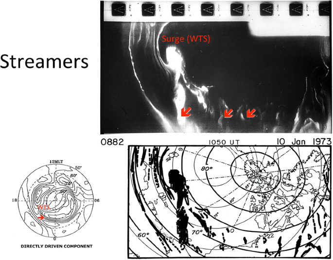

    

    An example of DMSP images of a westward traveling surge and associated streamers. Note that there is no streamer in the polar cap, indicating that streamers do not occur in the main part of the polar cap. The average DD current pattern is also shown to indicate the western end of the electrojet which is the head of westward traveling surges

Concluding remarks

In this paper, it is shown that the “current lines” approach suggested by Alfven et al. (1967) has given us some quantitative understanding of the input–output relation and the associated flow of energy in causing auroral substorms.

It is emphasized here that the attempted synthesis is only a first attempt based on what we have learned so far. It is hoped that the requirements needed to explain the expansion phase are at least useful for future studies, regardless of theories to explain the expansion phase.

Obviously, however, all the quantities presented here are very tentative ones, and they may not be totally consistent among them. Thus, the purpose of this paper is in part to emphasize the need for a quantitative input–output approach and the “current lines” approach, instead of “magnetic field lines” approach, in studying auroral substorms.

References

Ahn B-H, Akasofu S-I, Kamide Y (1983) The Joule heat production rate and the particle energy injection rate as a function of the geomagnetic indices AE and AL. J Geophys Res 88:62756. doi:10.1029/JA088iA08p0675
Ahn B-H et al (1989) The auroral energy deposition over the polar ionosphere during substorms. Planet Space Sci 37:239. doi:10.1016/0032-0633(89)90022-6
Akasofu, S.-I., J. C. Cain and S. Champman (1961) The magnetic field of a model radiation belt, numercally computed. J Geophys Res 66:4013–4026.
Akasofu S-I (1964) The development of the auroral substorm. Planet Space Sci 12:273
Akasofu S-I, Chapman S, Mend C-I (1965) The polar electrojet. J Atmos Terr Phys 27:1301
Akasofu, S.-I. (1968) Polar and magnetospheric substorms, D. Reidel Pub. Co. Dordrecht-Holland, Holland.
Akasofu S-I (1981) Energy coupling between the solar wind and the magnetosphere. Space Sci Rev 28:121
Akasofu S-I (1992) A confirmation of the validity of the electric current distribution determined by a ground-bases magnetometer network. Geophys J Inst 109:191–196
Akasofu, S.-I., Exploring the Secrets of the Aurora, Springer, 2007.
Akasofu S-I (2003a) A source of auroral electrons and the magnetospheric current systems. J Geophys Res 108:2006. doi:10.1029/2002 JA009547 A4
Akasofu S-I (2003b) Chapman and Alfven: A rigorous mathematical physicist versus an inspirational experimental physicist, EOS, 84, 269–274.
Akasofu S-I, Meng C-I, Lui TY (2011) Importance of auroral features in the search for substorm onset processes. J Geophys Res 116:A02209. doi:10.1029/2010JA016079
Akasofu S-I (2013) Where is the magnetic energy for the expansion phase of auroral substorms accumulated? J Geophys Res 118:1–7. doi:10.1002/2013JA019042
Alfven, H (1967) The Birkeland Symposium on Aurora and Magnetic Storms, ed. by A. Egeland and J. Holtet, Centre National de la Recherche Scientific, 439–444
Alfven H (1977) Electric currents in cosmic plasmas. Rev Gephys And Space Phys 15:271–284
Alfven, H (1986) Double layers and circuits in astrophysics, IEEE Transaction on Plasma Science, Vol.PS-14, No. 6, 779–796
Angelopoulos V et al (2008) Tail reconnection triggering substorm onset. Science 321:931–933
Axford WI, Hines CO (1961) A unified theory of high-latitude geophysical phenomena and geomagnetic storms. Can J Phys 39:1433
Birn, J., K. Schinder and M. Hesse (2012) Magnetotail aurora connection: the role of thin current sheet, 337–346, in Auroral Phenomenology and magnetospheric processes: Earth and other planets, ed. by A. Keiling, E. Donovon, F. Bagenal and T. Karlsson, AGU Monograph 197. Washington, D.C.
Bostrom R (1964) A model of the auroral electrojet. J Geophys Res 69:4983–4999
Bostrom, R. (1974), Ionosphere-magnetosphere coupling, 45, in Magnetospheric physics, ed. by B. M. McCormac, Dordrecht, D. Reidel-Holland Publishing Co., Holland
Bristow WA, Jensen P (2007) A superposed epoch study of SuperDARN convection observations during substorms. J Geophys Res 112:A06232. doi:10.1029/2006JA012049
Cheng CZ (2004) Physics of substorm growth phase, onset and depolarization. Space Sci Rev 113:207
Coumans V, Blockx C, Gerard J-C, Hubert B, Connors M (2007) Global morphology of substorm growth phase observed by the IMAGER-SI12 imager. J Geophys Res 112:A11211. doi:10.1029/2007JA012329
Dungey JW (1961) Interplanetary magnetic field and the auroral zones. Phys Res Lett 6:7. doi.1103/PhysRevLett. 6, 47
Frank LA, Craven JD, Burch JL, Williams DJ (1982) Polar view of the earth’s aurora with Dynamic Explorer. Geophys Res Lett 9:1001
Ge YS, Russell CT (2006) Polar survey of magnetic field in near tail: reconnection rare inside RE. Geophys Res Lett 33:L02101. doi:10.1029/2005GL024574
Haerendel G (2007) Auroral arcs as sites of magnetic stress release. J Geophys 112:A09214. doi:10.1029/2007JA012378
Haerendel G (2008) Auroral arcs as current transformers. J Geophys Res 113:A07205. doi:10.1029/2007JA012947
Haerendel G (2009) Poleward arcs of the auroral oval; during substorms and the inner edge of the plasma sheet. J Gephys Res 114:A06214. doi:10.1029/2009JA014138
Henderson, M. G. (2009) Observational evidence for an inside-out substorm onset scenario, Ann. Geophys 27:2129–2140
Israelevich PL, Ershkovich AI, Oran R (2008) Current carriers in the bifurcated tail current sheet: ions or electrons. J Geopys Res 113:A04215. doi:10.1029/2007JA012541
Kamide Y et al (1982) Global distribution of ionospheric and field-aligned currets during substorms as determined from six IMS meridian chains of magnetometers: initial results. J Geophys Res 87(A10):8228–8240. doi:10.1029/JA087iA10po8228
Lui ATY, Kamide Y (2003) A fresh perspective of the substorm current system and its dynamo. Geophys Res Lett 30:1958. doi:10.1029/2003GL017835
Lui ATY (2011) Reduction of the cross-tail current during near-Earth depolarization with multisatellite observations. J Geophys Res 116:A12239. doi:10.1029/2010JA016078, doi:10. 1029/2011JA017107 (2011b),116, A03211
Lyons LR et al (2001) Timing of substorm signatures during the November 24, 1996, Geospace Environment Modeling event. J Geophys Res 106:349–359
Lyons LA, Nishimura Y, Shi Y, Zou S, Kim H-J, Angelopolous V, Heinselman C, Nicolls MJ, Fornacon K-H (2010) Substorm triggering by a new plasma intrusion: incoherent-scatter radar observations. J Geophys Res 115:A07223. doi:10.1029/2009JA015168
Machida S, Mukai T, Saito Y, Hirahara M, Obara T, Nishida A, Terasawa T, Maezawa K (1994) Plasma distribution functions in the earth’s magnetotail (XGSM ∼ −42 Re) at the time of a magnetospheric substorm: GEOTAIL/LEP observation. Geophys Res Lett 21(11):1027–1030
Nishimura Y, Lyons L, Zou S, Angelopoulos V, Mende S (2010) Substorm triggering by new plasma intrusion: THEMIS all-sky imager observations. J Geophys Res 115:A07222. doi:10.1029/2009JA015166
Ohtani S-I, Takahashi K, Lui ATY (2002) Electron dynamics in the current disruption region. J Geophys Res 107(A10):1322. doi:10.1029/2001JA009236
Perraut S, Ol C, Roux A, Park G, Chua D, Hoshino M, Mukai T, Nagai T (2003) Substorm expansion phase: observations from Geotail, polar and IMAGE network. J Geophys Res 108(A4):1159. doi:10.1029/2002JA009376
Shiokawa K, Yago K, Yumoto K, Baishev DG, Solovyev SI, Rich EJ, Mende SB (2005) Ground and satellite observations of substorm onset arc. J Geophys Res 110:A12225. doi:10.1029/2005JA011281
Sun W, Xu S-Y, Akasofu S-I (1998) Mathematical separation of directly-driven and unloading components in ionospheric equivalent currents during substorms. J Gephys Res 103(A6):11695–11700. doi:10.1029/97JA03458
Acknowledgements
I would like to thank all the magnetospheric physicists in the past and the present for their efforts in making a great progress in substorm research during the last 50 years. I owe especially Dr. Y. Kamide, Dr. Sun Wei, and Dr. B.-H. Ahn, A.T.Y. Lui, and C.-I. Meng for their long collaboration in pursuing the electric current/circuit approach.
I would like to dedicate this paper to Sydney Chapman and Hannes Alfven for their guidance during my early research life and also to Lou Frank for his great success in excellent imaging of auroral substorms.
Personal note
It may be worthwhile to mention why the four statements made by Alfven were mentioned in the introduction. It is because those statements have become the basis of this paper.
I met Hannes Alfven for the first time when Sydney Chapman asked me to join him to attend the Birkeland Symposium held in Norway in 1967. I heard about the great controversy between Chapman and Alfven (cf. Akasofu 2003b) by others before, so that I was a little apprehensive to meet Hannes. However, unexpectedly, he mentioned nothing about the debate. He was anxious to tell me that the concept of “frozen-in magnetic field lines” and “moving field lines” concepts should not be considered in studying auroral substorms and solar flares (except for solar interior); I told him that I have just begun to learn MHD from his book “Cosmical Electrodynamics”. He emphasized that I should take “current lines” approach, instead of “magnetic field lines” approach. His paper on this subject was published in the conference proceedings (which I quoted in this paper). I invited him to visit Alaska in 1974; at that time, he told me that his statements were realized in a study of the acceleration of auroral electrons; MHD does not allow for an electric field along magnetic field lines. Similarly, the breakdown of the “frozen-in magnetic field lines” condition (as observed during the expansion phase) may be essential in understanding the onset of the expansion phase.
When I met him a few times in Stockholm, he was complaining about my slow progress. However, in order to take the current lines approach, we had to set up six meridian chains of magnetometers to begin with. The analysis of the records required developing a few computer codes with my colleagues. It was as late as the end of 1990s, when we succeeded in separating DD and UL. Then, it took many more years to digest the results.
Unfortunately, the “current lines” approach has not been popular in our particular field, so much that many readers of this paper must encounter many unfamiliar terms, such as dynamo, power, circuits, inductance, and even the term electric currents for some. However, the “current lines” approach is one of the ways of studying substorms. Actually, the basis of this paper is not more than what is in physics 101, but the “current lines” approach has provided, I believe, some of the basic aspects of physics of auroral substorms, which has so far not been demonstrated by “the magnetic field lines” approach.
Author information
Authors and Affiliations
Corresponding author
Additional information
Competing interests
The author declares that he has no competing interests.
Rights and permissions
Open Access This article is distributed under the terms of the Creative Commons Attribution 4.0 International License (https://creativecommons.org/licenses/by/4.0), which permits use, duplication, adaptation, distribution, and reproduction in any medium or format, as long as you give appropriate credit to the original author(s) and the source, provide a link to the Creative Commons license, and indicate if changes were made.
About this article
Cite this article
Akasofu, SI. Auroral substorms as an electrical discharge phenomenon. Prog. in Earth and Planet. Sci. 2, 20 (2015). https://doi.org/10.1186/s40645-015-0050-9
Received:
Accepted:
Published:
DOI: https://doi.org/10.1186/s40645-015-0050-9