Observation of equatorial plasma bubbles by the airglow imager on ISS-IMAP

Abstract

Using 630 nm airglow data observed by an airglow imager on the International Space Station (ISS), the occurrence of equatorial plasma bubbles (EPBs) is studied. In order to examine the physical mechanisms in the boundary region between the Earth and the outer space, an ionosphere, mesosphere, upper atmosphere, and plasmasphere mapping (IMAP) mission had been conducted onboard the ISS since October 2012. The visible light and infrared spectrum imager (VISI) is utilized in the ISS-IMAP mission for nadir-looking observation of the earth’s atmospheric airglow. In this study, we automatically select EPBs according to the criterion for extracting the tilted dark lines from VISI data. Using the selected events, the dependence of the occurrence rate of EPBs is examined. There is no other report of the occurrence rate of EPBs using downward-looking visible airglow data (630 nm). In this result, the occurrence rate is high at all longitudes in the equinoctial seasons. In the solstice seasons, in contrast, the occurrence rate is very small especially in the Pacific and American sectors. This result is basically consistent with previous studies, e.g., those determined by plasma density data on DMSP satellites.During the June solstice in 2013, EPBs were observed in association with geomagnetic storms that occurred due to a southward turning of the IMF Bz. Using these events, we examined the storm-time features of the occurrence of EPBs in the Pacific-American sectors during the June solstice. In these sectors, where the occurrence rate of EPBs is very small during solstice seasons, some EPBs were observed in the peak and recovery phases of the storms. This result shows that the prompt penetration of electric fields causes the development of EPBs, in the data we analyzed, the geomagnetic storms did not inhibit the generation of EPB in the Pacific–American sectors.

Introduction

In the age of satellite-based communication, the study of equatorial plasma bubbles (EPBs) becomes ever more important. Radio signals from satellites scintillate and may often become disrupted due to irregularities of various scale sizes inside the EPBs. Therefore, since the early stages of EPB studies, observations using radio waves have been utilized, including radar observation (e.g., Woodman and LaHoz (1976); Kelley et al. (1981); Tsunoda et al. (1981)), ionosonde (e.g., Maruyama and Matsuura (1984); Abdu et al. (2003)), GPS scintillation (e.g., Pi et al. (1997); Otsuka et al. (2006); Brahmanandam et al. (2012)), and total electron content (TEC) fluctuation (Nishioka et al. (2008); Li et al. (2009)). Imaging of nighttime airglow has also been an effective method for the study of EPBs (e.g., Otsuka et al. (2002); Makela and Kelley (2003); Pimenta et al. (2003)). Since the plasma density decreases inside EPBs, the intensity of the airglow becomes depressed. The imaging observation from satellites are also utilized to examine the global structure of EPBs. The IMAGE satellite observed 135.6 nm airglow using a far-ultraviolet imaging system (FUV). Immel et al. (2003; 2004) showed that plasma depletions were observed by FUV data and that the drift speed of these depletion was of the order of 100 m/s. Similar observations were also done using a global ultraviolet imager (GUVI) on the TIMED satellite (e.g., Kil et al. (2004); Kamalabadi et al. (2009)). In this way, ultraviolet airglow observation is used for the satellite-based airglow observation, although the visual wavelengths, such as 630 nm and 777.4 nm, are used for the ground-based observations.

To study the climatological characteristics of EPBs, in situ observations also have been conducted. Defense Meteorological Satellite Program (DMSP) satellites track the sun-synchronous orbits at the altitude of 840 km and provide the in situ plasma density data. Huang et al. (2001) showed that the occurrence rate of EPBs is maximum in the equinoctial seasons, which is in general agreement with most ground-based observations. Burke et al. (2004), followed by Gentile et al. (2006), showed the seasonal-longitudinal distributions of the occurrence rate of EPBs. In their results, the occurrence rate became larger where the difference between the declination and the terminator angles at the magnetic equator was smaller. As for the solar activity dependence, it was clear that the occurrence rate increased with solar activity (e.g., Gentile et al. (2006); Xiong et al. (2010)).

As compared to the clear dependence of the occurrence rate of EPBs on long-term solar activity, the effect of geomagnetic storms on the occurrence of EPBs has been a subject of considerable discussion. Rastogi et al. (1981) showed that the scintillations due to EPBs in the postsunset decreased with magnetic activity. Using DE2 data, Palmroth et al. (2000) also showed that plasma density depletions were suppressed by geomagnetic activity. These results are consistent with the calculation results by the TIEGCM model (Carter et al. 2014a, b). In contrast, several recent studies showed that geomagnetic storms enhanced the EPB occurrence (Abdu et al. 2003; Kil and Paxton 2006; Li et al. 2006; Basu et al. 2007). During geomagnetic storms, the ionospheric electric field was affected by the prompt penetration electric field (e.g., Basu et al. (2007); Kikuchi et al. 2008) and disturbance dynamo (Blanc and Richmond 1980). During the main phases of the storms, the direction of the prompt penetration electric field is eastward in the dayside and dusk hours, which enhanced the growth rate of the Rayleigh-Taylor instability. In the recovery phase, this direction becomes opposite due to the over-shielding effect. The polarity of the disturbance dynamo is almost the same as the over-shielding electric field during the recovery phase (Abdu et al. 2008). However, the effect of the disturbance dynamo is delayed as compared to the prompt penetration electric field and last longer. The EPB occurrence is determined by the competing effects of these electric field.

The ionosphere, mesosphere, upper atmosphere, and plasmasphere mapping (IMAP) mission is a part of the Japanese Experiment Module (JEM) second stage plan on the International Space Station (ISS). In order to make nadir-looking spectroscopic measurement of airglows, a visible imaging spectrometer instrument (VISI) was installed on the ISS-IMAP. The target for airglow emissions in this study is the 630 nm band. The 630 nm airglow is emitted by the dissociative recombination of atomic oxygen. The emission layer of the airglow is at the height of 250 km, and the intensity of the airglow reflects the density of the ionospheric plasma. As compared to the other satellites, the altitude of the orbit is lower (about 400 km), which is an advantage for airglow observation in that the attenuation of the airglow becomes smaller. Since the orbital period and inclination of the ISS are 91 min and 51.64°, respectively, the ISS tracks the whole earth in 1 day. Therefore, the climatology of the EPB occurrence can be determined using VISI data. In this study, a method for automatic determination of EPBs is used to generate the global map of the occurrence rate of EPBs. This study provides statistical results for the EPB occurrence using nadir-looking imaging data (630 nm), which has been never reported. It is very important to compare the statistical results with other observational results in order to examine the characteristics of these data.

With the results from this global map, however, the enhancement of the EPB occurrence, which is inconsistent with previous studies, appeared. The cause of this inconsistency, namely, the effect of geomagnetic storms, is discussed.

Methods/Experimental

Data

The ISS consists of a number of modules and components. The Japan Aerospace Exploration Agency (JAXA) is one of the participating space agencies and provides the largest single module on the ISS, the Japanese Experiment Module (JEM), called “Kibou.” The IMAP mission was one of the onboard missions installed in the Exposed Facility Unit on Kibou. This mission utilized the VISI for airglow observation. The observed wavelengths of the VISI were 730 nm (OH Meniel band), 762 nm (O₂(0-0)), and 630 nm (OI). To examine the occurrence of EPBs, the 630 nm airglow data, which is a good proxy for the electron density at an altitude of 250 km, is used in this study. The VISI faced the Earth’s surface and had two slits directed forward and backward at 45° from the nadir. The angle of the field of view (FOV) perpendicular to the orbit is 90°, which is 300 km in width at the altitude of 250 km (Sakanoi et al. 2011). The intensity of the airglow is extracted by the differential of the two wavelengths (630 nm and the background). This is because the streetlights and the reflections of moonlight on clouds near the full moon contaminate the airglow intensity. In this study, the EPB occurrence was examined by using 630 nm forward-slit data observed from September 2012 to April 2014. Figure 1 shows a sample of the 630 nm airglow data along the track of the ISS observed at 02 UT on 25 September 2012. The bright region around 15° to 30° in geographic latitude is due to the equatorial ionospheric anomaly (EIA). Several dark lines are recognized in EIA. Such dark lines in the VISI image are EPBs, in which the electron density is depressed as compared to the background.

Fig. 1

The 630 nm airglow image along the track of the ISS observed at 02 UT on 25 September 2012

Detection of EPBs

Because the size of the FOV is narrower as compared to the scale of the EPBs, the EPBs are recognized as dark lines in the VISI data. These lines are usually tilted to the track with various angles as shown in Fig. 2a, which is the same data in the airglow image shown in Fig. 1. In order to manage a large amount of image data, automatic detection of EPBs is required. To select the EPBs from the VISI data, we developed the following criteria. A schematic figure of these criteria is shown in Fig. 2c.

• (i) Split a part of image into 3 ×3 bins, each bin having a size of 6 ×21/22 pixels.

  Fig. 2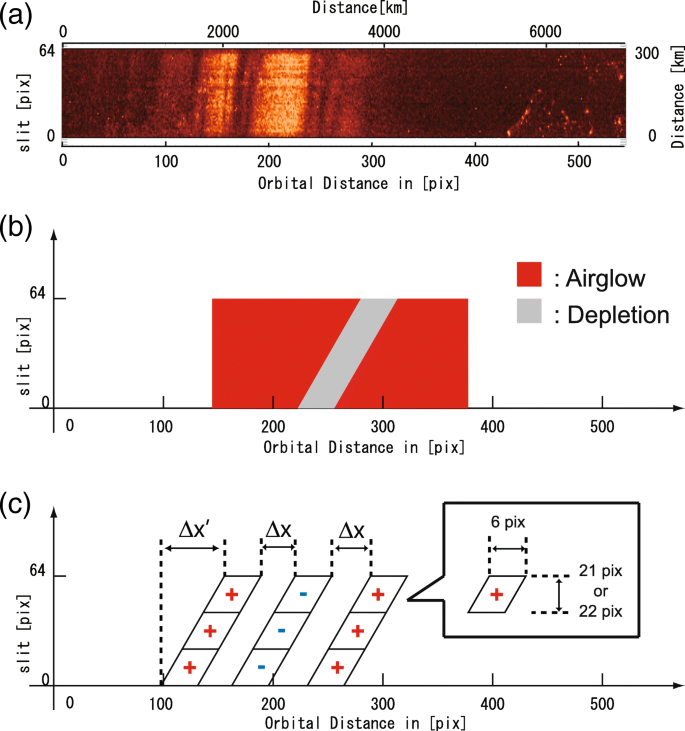

  

  The schematic figure of the selection of the EPB events. The top panel a shows the airglow image obtained on 25 September 2012. The middle panel b shows the model image of the tilted EPB as shown by an arrow in the top panel. To detect this EPB, the spatial variations of the airglow shown in the bottom panel c were sought

• (ii) Calculate the average intensity of each bin.

• (iii) When the average intensities of three bins perpendicularly adjacent to the track (the bins noted by “ −” in Fig. 2c) are 10% less than the leading and trailing bins (the bins noted by “+”), select these bins as the occurrence of an EPB.

• (iv) In calculating the average intensity, vary the gap to the leading and trailing bins (Δx in Fig. 2c) from 0 to 6 pixels.

• (v) To pick the tilted dark lines, tilt the shapes of the bins by Δx^′ as shown in Fig. 2c. In this study, Δx^′ = 6n (n=1, 2, ⋯ 10). In selecting an EPB, the same procedures given in (iii) and

• (iv) are applied.

The width of the bin in the moving direction is 6 pixels. The actual scale of this width corresponds to 70 to 80 km, depending on the path. This means that these criteria can pick larger scale EPBs. In the original plan of the IMAP, the VISI was designed to detect a 10% variation in the total intensity for each airglow emission assuming that the typical total intensity of the 630 nm airglow is 100 R with no background emission and that the sensitivity of the VISI is 0.028 el/R/pixel/s (Sakanoi et al. 2011). In the real laboratory test, in contrast, the sensitivity of the VISI is 0.032 el/R/pixel/s. The signal to noise ratio (S/N ratio) of CCD is determined as $S/\sqrt {S+N_{bk}+N_{ro}^{2}}$ where S is the number of counts for the target (airglow), N_bk is the number of counts for background, and N_ro is read-out noise. Because the exposure time is 1 s and the row-column binning on CCD is 1 ×16 pixels, S for 100 R is 0.032 ×100×1×16 = 51.2 counts. The value of N_ro is estimated as 2 in the laboratory test. Therefore, S/N ratio is $51.2/\sqrt {51.2+35.8+2^{2}} = 5.3$ when the total intensity is 100 R and the background intensity is 70 R (N_bk=0.032×70×1×16 = 35.8). In addition, the average value of the airglow in 6 ×21/22 pixels of the airglow image is used to evaluate the depression of the airglow. Therefore, the S/N ratio of the VISI is large enough to detect the depression of the airglow due to EPBs.

Using this criterion, we selected 413 events of EPBs from September 2012 to April 2014. Some events that are not EPBs were also detected using this criteria because of the scattering of moonlight by clouds and city lights. By checking the background images, these false detections were removed by visual inspection. Therefore, depletions in airglow intensity other than those due to EPBs were not selected in this study, while some weak EPBs and the edges of EPBs were also not selected.

Results

Occurrence rate of EPBs

Selecting EPB events based on the criteria as described in the previous section, the occurrence rate of EPBs is determined. As the EPBs are developed around the equatorial region, only the observation region around the equator is considered. Since the inclination of the ISS orbit is 51.64°, the ISS sweeps at this angle around the equator. Since the airglow observation was done only in the night time and thus was affected by the phase of the moon, the latitude of the observation region is dependent on day of year. Considering this situation, we have calculated the occurrence rate of EPBs in each bin using the ratio of the number of EPBs to the observation duration where the magnetic latitude is within 30° in geographical coordinates.

Figure 3 shows the occurrence rate of EPBs using the VISI airglow imager data. The horizontal and vertical axes show geographical longitude and month, respectively. In determining the occurrence rate, the number of EPBs and the observation duration were counted in each bin with 15° in longitude × 10 days. Then, the occurrence rate is determined by the number of EPBs per hour in each bin.

Fig. 3

The occurrence rate of EPBs observed by the VISI data

As for the global occurrence distribution of EPBs, Burke et al. (2004) and Gentile et al. (2006) determined similar occurrence maps using the DMSP satellites. In their studies, the EPB occurrence was determined by the fluctuations in the plasma density profiles (Huang et al. 2001). The basic characteristics of the occurrence rate in this study are almost the same as in their results: (i) the occurrence rate is high in the equinox seasons, (ii) the occurrence rate is highest during the December solstice in the Atlantic sector (300–360° longitude) and African sector (0–30°), (iii) around the June solstice, the occurrence rate is low in the Atlantic sector and Indian sector (60–150°). It is worth noting that the observation altitude of the DMSP satellite (840 km) is higher than that of the VISI. In contrast, the observation of EPBs in the VISI data requires that the background 630 nm airglow is rather bright. As shown in Fig. 1, this condition is usually met around the EIA, whose geomagnetic latitude is about 10° to 25°. EPBs are generated around the magnetic equator and develop to higher altitudes. Assuming that EPBs elongate along the magnetic field lines, the highest altitude of EPBs observed by the VISI seems to be larger than 500 km in the equatorial plane. This means that the VISI observes the EPBs that have developed to some extent. The altitude of the DMSP satellites is 840 km, independent of latitude. These DMSP observations also correspond to well developed EPBs. From these facts, the seasonal and longitudinal dependence of the occurrence of EPBs determined by the VISI is almost the same as that of DMSP satellites as shown in Burke et al. and Gentile et al. However, the difference in the observation altitudes between the DMSP and the IMAP is reflected in the absolute value of the occurrence rate. This will be discussed later. It is also noticed that the occurrence rate in the Pacific–American sector (200–300° in longitude) around the June solstice is enhanced in this study, while it is very low in the DMSP results. As described later, it is considered that the main reason for this difference is consecutive EPB events during geomagnetic storms. In addition, the under developed EPBs indicated by Makela et al. (2004) may contribute to this difference. In the next section, we look at the relationship between these consecutive events and the geomagnetic storms. The effect of under developed EPBs will be also discussed later.

EPBs during geomagnetic storms

Although Solar cycle 24 is a period of weaker solar activity, many geomagnetic storms occurred in 2013 since it was the local minimum between the peaks in 2012 and 2014. In June and July 2013, six storms occurred as shown in Table 1. In this table, the geomagnetic storms whose minimum Dst is less than − 50 nT are listed. In association with these storms, VISI observations were carried out except for storm S2. As described previously, the data of background emission intensity are necessary to detect EPBs. Unfortunately, the background emissions were not identified in storms S4 and S5. In the remaining three storms (S1, S3, and S6), the detection of EPBs during geomagnetic storms was examined. Table 2 shows a list of the EPBs automatically detected in June and July 2013. Figure 4 shows the locations of these EPBs and corresponding VISI images mapped along the ISS orbits. In Table 2, the storm-associated events are EPBs #1 and #5–14. These events correspond to storms S1 and S3. Regarding the event associated with storm S6, EPB #15 might be a prospective candidate. However, storm S6 started at 20 UT on July 13 just after the occurrence of EPB #15. Therefore, there is no event associated with storm S6. Here, we checked the events left over from the automatic selection of the EPBs. Figure 5 shows the VISI image on 15 July 2013. We recognize an event in the African sector as shown by a circle. In this event, the tip of an EPB appeared. In the next orbit, the slight depletion of the airglow is also recognized. Including these additional events, EPBs were excited in association with all storms in which the observation of EPBs is feasible. Therefore, we can say that the storms do not inhibit the occurrence of EPBs.

Fig. 4

The EPB events occurring between June and July 2013, and the associated airglow images along the ISS-tracks. The locations of EPBs are shown by crosses. Blue crosses show the events on 29 June 2013. The red and blue numbers show the start and end times of the observation of each track, respectively

Fig. 5

The airglow images along the ISS-tracks obtained on 15 July 2013. The blue numbers indicate the end time of the observations of each track

Table 1 The magnetic storms that occurred during June–July 2013

Table 2 A list of EPBs detected during June–July 2013

The events that occurred in the Pacific–American sector in association with storm S3 are shown by blue crosses in Fig. 4. These occurrences cause the difference in the occurrence rate between the present result and DMSP results. Note that EPBs #5–10 (listed in Table 2) that occurred in the Pacific-American sector were detected in four consecutive paths of the ISS. The path of the ISS shifts westward while the EPBs usually drift eastward. During storms, the EPBs may drift westward (e.g., Abdu et al. (2003); Sobral et al. (2011); Santos et al. (2016)). The longitudinal distances between the EPBs observed on 29 June are about 20° or 2200 km. If it is assumed that these EPBs are the same events observed in the different paths, the drift speed of the EPBs is about 400 m/s, which is too fast for drift speed. Therefore, it is confirmed that EPBs #5–10 are not the same events but individual events. Since the EPB occurrence is very low during the June solstice in the Pacific–American sector, these events are very noticeable. In Fig. 6, the solar wind parameters (solar wind speed and IMF-Bz) and the geomagnetic index (AU/AL and SYM-H) from 28 to 30 June are shown. The determination of the SYM-H index is almost the same as that of Dst index, although the SYM-H index is a 1 min value (Iyemori 1990). In this storm, the IMF Bz turned to the south at 07 UT on 28 June and maintained a southward direction until 11 UT on 29 June. During this period, the magnetic flux on the dayside moved tailward due to the magnetic reconnection. Then, the accumulation of the magnetic flux in the magnetotail triggered the reconnection in the tail. The storm started after the southward turning of the IMF Bz and reached its peak around 06 UT on 29 June. Just after the peak, the storm turned into the recovery phase. By the end of 30 June, the storm reached almost steady state. In association with the variation of the SYM-H index, the polar regions were also in a magnetically disturbed condition. The occurrence of EPBs #5–10 are shown by the vertical arrow in association with the variation of the SYM-H index. These EPBs were observed around the peak of this magnetic storm (the arrows for EPBs #5 and #6 and those for #9 and #10 overlap, respectively). In addition, EPBs were observed in the recovery phase of the storm on the next day (EPBs #13 and #14).

Fig. 6

The temporal variations of solar wind parameters and the geomagnetic index during 28–30 June 2013. From top to bottom, solar wind speed, IMF Bz, AU/AL index, and SYM-H index are shown. In the AU/AL index panel, the positive and negative values show the AU and AL index, respectively. In the bottom panel, the occurrence of EPBs listed in Table 2 are shown

Discussion

In the previous section, EPBs were observed by the VISI data during the geomagnetic storms with high probability. Though there has been controversy over the relationship between geomagnetic storms and the occurrence of EPBs, many recent studies have shown that EPBs occur during geomagnetic storms. Using GPS observation, Basu et al. 2001showed that scintillations were observed over western South America around the peaks of geomagnetic storms during the equinox seasons. In the Brazilian sector, an EPB event was initiated in the dusk sector by prompt penetration of the magnetospheric electric field even though a disturbance dynamo was expected to be active (Abdu et al. 2003). Li et al. (2010) also showed that the variations in TEC occurred over a wide longitudinal range associated with geomagnetic storms. Combining DMSP plasma density observations with ROCSAT-1 satellite observations, Kil and Paxton (2006) showed that plasma density depletions and irregularities were observed during a geomagnetic storm. These studies show that geomagnetic storms cause the development of EPBs.

Usually, the equatorial electric field, which contributes to the development of EPBs, may be perturbed in association with many geomagnetic indices. When the IMF Bz is southward, the magnetic reconnection occurs in the dayside of the magnetosphere. As the magnetic fluxes are transported to the magnetic tail, the magnetic reconnection also occurs in the magnetic tail. In this process, the electric field entered at the polar region penetrates toward the low latitudes. In the dusk ionosphere, this penetrating electric field (PE) is eastward and causes the plasma bubbles to grow (e.g., Abdu et al. 2009). This enhancement of the PE is shown by both of calculation and observation. For example, the numerical simulation by Huba et al. 2005 showed the increase in the E ×B drift due to enhancement of the eastward electric field. Rice Convection Model simulations suggest the penetration of the electric field during the growth phase of a magnetic storm (Spiro et al. 1988; Fejer et al. 1990). Jicamarca radar observations also show the enhancement of vertical drift of the ionospheric plasma (Huang 2011). During the recovery phases of storms, in contrast, the region 2 shielding current develops and the over-shielding effect dominates (e.g., Kelley et al. (1979); Kikuchi et al. 2008). The opposite polarity of the electric field increases in this situation. Therefore, this implies that the electric field in the recovery phase inhibits the EPB occurrence (e.g., Huang et al. 2001; Abdu et al. 2009).

In addition to the PE, the disturbance dynamo electric field (DD) also affects the ionospheric electric field in the equatorial region during storms. As the polarity of the DD electric field is almost the same as that of the PE in the recovery phase (e.g., Richmond et al. (2003)), the effect of the DD may suppress the EPBs in the evening or post sunset hours. As for the appearances of both PE and DD electric fields, Maruyama et al. (2005) also calculated the vertical E ×B drift speed of the ionospheric plasma. In their results, at the later stage of a storm, the high latitude magnetospheric sources of ion convection and auroral precipitation affect the global neutral wind field and the ionospheric conductivities. Then, the PE effect is reduced and the development of the DD is also affected. This means that the electric field affected by both the PE and DD is not the simple summation of the PE and DD effects, and the effect of the DD cannot be estimated independently. However, it is interesting that the enhancement of the vertical drift in the pre-reversal enhancement (PRE) reaches almost the same value whether the effect of the DD is considered or not. Surely, the appearance of the effect of the DD must be carefully examined; however, it is possible that the effect of DD is not large enough to inhibit the occurrence of EPBs. In addition to the effect of the electric field, the specific feature of this storm is a highly fluctuating polar electric field as shown in the AE index from 12UT on 28 June to 12UT on 29 June. Even during the event on 26–27 August 1998 as shown in Abdu et al. (2003), the AE index was quite disturbed, and EPBs were observed in the Brazilian sector. As noted in their study, sustained AE activity contributes to the generation of EPBs, which may contribute to the consecutive events during the storm.

During storm S3, EPBs #13 and #14 shown in Table 2 occurred in the recovery phase of the storm. In the previous studies concerning EPBs in the recovery phase, the enhancement of the S4 index was observed during postmidnight period in the African and South American region in the 2015 St. Patrick’s Day storm Carter et al. 2016. In association with an intense storm, the density variations in the early morning were observed by the C/NOFS satellite (Zhou et al. 2016). Comparing these previous studies, EPBs #13 and #14 were observed before midnight, which is the typical time zone for an EPB occurrence. As previously described, EPBs observed around premidnight during the recovery phase are rare. Therefore, the occurrence of EPBs #13 and #14 seems to be affected by some unusual circumstances. One possibility is the fluctuation of the IMF Bz. As shown in Fig. 6, at the occurrence of EPBs #13 and #14, the IMF Bz was highly fluctuating. Generally, the over-shielding effect appears during the recovery phase of the storm due to a northward IMF following a southward IMF. In this case where the IMF Bz is fluctuating, it is possible that the over-shielding effect does not appear clearly. Therefore, the enhancement of the eastward electric field still continues at some level, and the occurrence of the EPBs is not inhibited, even in the recovery phase.

In the previous section, we have shown that the occurrence rate of EPBs determined by the VISI is similar to those determined by the DMSP satellites, although the observation altitudes are different. However, it is possible that the difference in the observation altitudes between the DMSP and the IMAP is reflected in the absolute value of the occurrence rates. Gentile et al. (2006), in which the occurrence rates of EPBs were determined by DMSP data, examined individual plasma density profiles acquired within ± 20° with respect to the magnetic equator during all DMSP satellite passes at local times greater than 19:30. They examined EPB encounters in a particular pass. Subsequently, the occurrence rate of EPBs was calculated by the ratio of the number of orbits with EPBs divided by the total number of orbits in each bin. As shown in Figs. 1 and 2 in Gentile et al. (2006), the maximum rates were approximately 70% and 50% around the Atlantic–African sectors in 1989–1992 and 1999–2002, respectively. On the other hand, the occurrence rate in this study was determined by the number of EPBs per hour. To compare the present results with those of Gentile et al. (2006), we converted the number of EPBs per hour to EPBs per orbit. In this study, the number of EPBs and the observation duration were counted within a strip of 60° latitude, which extended from 30°S to 30°N in geographic latitude, in a bin with 15° in longitude and 10 days duration. The total duration of a bin corresponds to that of the orbital element of the 60° latitude range, in hours, multiplied by the total number of orbits during 10 days (calculated for each of 15° longitude intervals). The occurrence rate estimated in the present result as 1.8 per hour, in fact corresponds to the total number of EPBs observed in all the orbital elements (each of 60° range in each orbit) of the bin. Therefore, the occurrence rate as shown in Fig. 3 corresponds to the total number of EPBs observed in all the orbital elements of the bin. Each such orbital element has a duration of a fraction of the orbital period of 101 min. This fraction is 60°/360° ×101 min = 16.8 min. 1 h therefore contains 60/16.8 = 3.6 orbital elements. As a result, the number of EPB per orbit is 1.8/3.6 = 0.5, i.e., the occurrence rate is approximately 50%, which corresponds to the maximum rate obtained by DMSP in 1999–2002 as shown in Fig. 2 in Gentile et al. (2006). As discussed by Gentile et al. (2006), the occurrence rate of EPB is dependent on the sunspot number. In the periods of 1999–2002 and 2012–2014, the monthly averages of the sunspot number were about 250 and 150, respectively. Therefore, the maximum of the occurrence rate in the present study, which examined the data obtained in 2012–2014, would be smaller than that determined by the DMSP. Since the observation altitude by the IMAP (250 km) is lower than that by the DMSP (840 km), on the other hand, it is expected that the occurrence rate of the present result would be larger than that of the DMSP. In view of the effects of both the sunspot number and the observation altitudes, the occurrence rates of the present study and that determined by the DMSP are comparable.

As for the difference of the distribution of the occurrence rate, the occurrence rate in the Pacific–American sector (200–300° longitude) around the June solstice is enhanced in this study, while it is very low in the DMSP results. Consecutive EPB events occur in this sector in association with magnetic storms during June–July in 2013. Considering the geomagnetic condition as shown in the previous section, it is believed that these consecutive events occur due to the geomagnetic storms. In contrast, the observational results in the lower equatorial region as shown in Makela et al. (2004) may have a relationship with the difference in the occurrence map in the Pacific–American sector. In Makela et al. (2004), dual airglow imaging systems, Cornell All-Sky Imager (CASI) and the Cornell Narrow-Field Imager (CNFI), are used. These systems are located in Maui Island, Hawaii. The FOV of CASI and CNFI cover the higher and lower latitudinal regions, respectively. The CASI observes over a circular region whose geographic latitude spreads over 13 to 28° in geographic latitudes. The FOV of CNFI is directed to the south with a look-angle of 17.9° elevation and covers the equatorial region with geographic latitudes of 3 to 18°. In mapping their FOVs to the magnetic equatorial plane, the altitudes of the FOV of CNFI and CASI in the equator are 400 km to 1000 km and 700 km to 2500 km, respectively. A schematic figure of the relationship of these FOV altitudes is shown in Fig. 7. In this figure, the emission layer is assumed to be at the altitude of 300 km, as shown in Makela et al. (2004). Using imager data obtained by CNFI and CASI, the occurrence rates of EPBs in both regions are obtained. In the higher latitudinal region, the occurrence is high in the equinox seasons, which is almost the same as in the previous studies. In the lower latitudinal region, in contrast, the occurrence rate is also high in the June solstice season in addition to the equinox seasons. This result indicates that EPBs whose altitudes in the equatorial plane are smaller than 700 km are often generated around the June solstice. Because the IMAP can observe the EPBs that occur around the equatorial anomaly, these smaller EPBs are observable from the IMAP. As shown in Table 2, the geomagnetic latitudes of several events that are considered to be excited by the geomagnetic storms are less than 16°. Based on the results of Makela et al. (2004), these events may occur without geomagnetic storms. However, the latitudes for some events, e.g., EPB #9 and #14, are larger than 16°, implying that the geomagnetic storm surely affected the development of these EPBs as discussed previously. In the present study, it is possible that the enhancement of the occurrence rate of EPBs in the Pacific–American sector during the June solstice is due to the geomagnetic storms. However, the number of EPBs observed by the VISI (413 events) is much less than that by the DMSP (14 412 events) (Gentile et al. 2006). Because the number of EPB in each bin is also small, the occurrence map determined in the present study is easily affected by additional events generated for any reasons. In order to determine the differences in the occurrence map in detail, further longer observations of airglow are required.

Fig. 7

The altitudes of EIA and FOVs of CASI and CNFI in the equatorial plane and their latitudinal locations mapping along the field lines

Conclusions

In this study, the EPB occurrence is examined using nadir-looking 630 nm airglow data observed by the VISI imager on the ISS-IMAP during 2013–2014. Based on the criteria for selecting EPBs, EPBs were automatically detected. The occurrence rate of EPBs determined in this study is consistent with previous studies. Even though several EPBs were missed due to the automatic detection, the distribution of the occurrence rate is almost the same as in the previous solar maximum periods. In contrast, the absolute value of the occurrence rate of EPBs in this study is larger than those determined by the DMSP satellites. This is explained by the difference in the observation altitudes. Moreover, the occurrence rate determined in this study is somewhat higher in the Pacific and American sectors around the June solstice, which is different compared to previous studies. The cause of this difference is the consecutive EPB events observed in association with geomagnetic storms. It is possible that the prompt penetrating electric field, which enhances during storms, favors the occurrence of EPBs in this sector. However, the imager observation near the magnetic equator from Maui Island as shown in Makela et al. (2004) showed the enhancement of the occurrence rate around the June solstice. This result may have a relationship with the difference. Further, imager observation from space is necessary in order to examine the difference in the occurrence rate.

Even though the criteria for EPB detection proposed in this study select a number of events from the VISI data, some complicated events are missed. To detect EPBs more accurately, it is necessary to capture the intensity profile of the airglow after removing contamination and other noise sources, such as city lights and the reflection of the moon light from the clouds. Further investigation of the occurrence of EPB will help the progress of projects imaging the boundary regions between the Earth and outer space.

References

Abdu, MA, Batista IS, Takahashi H, MacDougall J, Sobral JH, Medeiros AF, Trivedi NB (2003) Magnetospheric disturbance induced equatorial plasma bubble development and dynamics: a case study in Brazilian sector. J Geophys Res 108:1449. https://doi.org/10.1029/2002JA009721.
Abdu, MA, de Paula ER, Batista IS, Reinisch BW, Matsuoka MT, Camargo PO, Veliz O, Denardini CM, Sobral JHA, Kherani EA, de Siqueira PM (2008) Abnormal evening vertical plasma drift and effects on ESF and EIA over Brazil-South Atlantic sector during the 30 October 2003 superstorm. J Geophys Res 113:A07313. https://doi.org/10.1029/2007JA012844.
Abdu, MA, Kherani EA, Batista IS, Sobral JHA (2009) Equatorial evening prereversal vertical drift and spread F suppression by disturbance penetration electric fields. Geophys Res Lett 36:L19103. https://doi.org/10.1029/2009GL039919.
Basu, S, Basu S, Valladares CE, Yeh H-C, Su S-Y, MacKenzie E, Sultan PJ, Aarons J, Rich FJ, Doherty P, Groves KM, Bullett TW (2001) Ionospheric effects of major magnetic storms during the International Space Weather Period of September and October 1999: GPS observations, VHF/UHF scintillations, and in situ density structures at middle and equatorial latitudes. J Geophys Res 106:30389–30413. https://doi.org/10.1029/2001JA001116.
Basu, S, Basu S, Rich FJ, Groves KM, MacKenzie E, Coker C, Sahai Y, Fagundes PR, Becker-Guedes F (2007) Response of the equatorial ionosphere at dusk to penetration electric fields during intense magnetic storms. J Geophys Res 112:A08308. https://doi.org/10.1029/2006JA012192.
Blanc, M, Richmond AD (1980) The ionospheric disturbance dynamo. J Geophys Res 85:1669–1686.
Brahmanandam, PS, Uma G, Liu JY, Chu YH, Latha Devi NSMP, Kakinami Y (2012) Global S4 index variations observed using FORMOSAT-3/COSMIC GPS RO technique during a solar minimum year. J Geophys Res 117:A09322. https://doi.org/10.1029/2012JA017966.
Burke, WJ, Huang CY, Gentile LC, Bauer L (2004) Seasonal-longitudinal variability of equatorial plasma bubbles. Ann Geophys 22:3089–3098. https://doi.org/10.5194/angeo-22-3089-2004.
Carter, BA, Yizengaw E, Retterer JM, Francis M, Terkildsen M, Marshall R, Norman R, Zhang K (2014a) An analysis of the quiet time day-to-day variability in the formation of postsunset equatorial plasma bubbles in the Southeast Asian region. J Geophys Res 119:3206–3223. https://doi.org/10.1002/2013JA019570.
Carter, BA, Retterer JM, Yizengaw E, Groves K, Caton R, McNamara L, Bridgwood C, Francis M, Terkildsen M, Norman R, Zhang K (2014b) Geomagnetic control of equatorial plasma bubble activity modeled by the TIEGCM with Kp. Geophys Res Lett 41:5331–5339. https://doi.org/10.1002/2014GL060953.
Carter, BA, Yizengaw E, Pradipta R, Retterer JM, Groves K, Valladares C, Caton R, Bridgwood C, Norman R, Zhang K (2016) Global equatorial plasma bubble occurrence during the 2015 St. Patrick’s Day storm. J Geophys Res 121:894–905. https://dpi.org/10.1002/2015JA022194.
Fejer, BG, Spiro RW, Wolf RA, Foster JC (1990) Latitudinal variation of perturbation electric fields during magnetically disturbed periods: 1986 SUNDIAL observation and model results. Ann Geophys 8:441–454.
Gentile, LC, Burke WJ, Rich FJ (2006) A climatology of equatorial plasma bubbles from DMSP 1989-2004. Radio Sci 41:RS5S21. https://doi.org/10.1029/2005RS003340.
Huang, CS (2011) Occurrence of Equatorial Plasma Bubbles during Intense Magnetic Storms. Int J Geophys:401858. https://doi.org/10.1155/2011/401858.
Huang, CY, Burke WJ, Machuzak JS, Gentile LC, Sultan PJ (2001) DMSP observations of equatorial plasma bubbles in the topside ionosphere near solar maximum. J Geophys Res 106:8131–8142. https://doi.org/10.1029/2000JA000319.
Huba, JD, Joyce G, Sazykin S, Wolf R, Spiro R (2005) Simulation study of penetration electric field effects on the low- to mid-latitude ionosphere. Geophys Res Lett 32:L23101. https://doi.org/10.1029/2005GL024162.
Immel, TJ, Mende SB, Frey HU, Peticolas LM, Sagawa E (2003) Determination of low latitude plasma drift speeds from FUV images. Geophys Res Lett 30:1945. https://doi.org/10.1029/2003GL017573.
Immel, TJ, Frey HU, Mende SB, Sagawa E (2004) Global observations of the zonal drift speed of equatorial ionospheric plasma bubbles. Ann Geophys 22:3099–3107. https://doi.org/10.5194/angeo-22-3099-2004.
Iyemori, T (1990) Storm-time magnetospheric currents inferred from mid-latitude geomagnetic field variations. J Geomagn Geoelectr 42:1249–1265. https://dx.doi.org/10.5636/jgg.42.1249.
Kamalabadi, F, Comberiate JM, Taylor MJ, Pautet PD (2009) Estimation of electron densities in the lower thermosphere from GUVI 135.6 nm tomographic inversions in support of SpreadFEx. Ann Geophys 27:2439–2448. https://doi.org/10.5194/angeo-27-2439-2009.
Kelley, MC, Fejer BG, Gonzales CA (1979) An explanation for anomalous equatorial ionospheric electric fields associated with a northward turning of the interplanetary magnetic field. Geophys Res Lett 6:301–304. https://doi.org/10.1029/GL006i004p00301.
Kelley, MC, Larsen MF, LaHoz C, McClure JP (1981) Gravity wave initiation of equatorial spread F: A case study. J Geophys Res 86:9087–9100. https://doi.org/10.1029/JA086iA11p09087.
Kikuchi, T, Hashimoto KK, Nozaki K (2008) Penetration of magnetospheric electric fields to the equator during a geomagnetic storm. J Geophys Res 113:A06214. https://doi.org/10.1029/2007JA012628.
Kil, H, Su S-Y, Paxton LJ, Wolven BC, Zhang Y, Morrison D, Yeh HC (2004) Coincident equatorial bubble detection by TIMED/GUVI and ROCSAT-1. Geophys Res Lett 31:L03809. https://doi.org/10.1029/2003GL018696.
Kil, H, Paxton LJ (2006) Ionospheric disturbances during the magnetic storm of 15 July 2000: Role of the fountain effect and plasma bubbles for the formation of large equatorial plasma density depletions. J Geophys Res 111:A12311. https://doi.org/10.1029/2006JA011742.
Li, G, Ning B, Wan W, Zhao B (2006) Observations of GPS ionospheric scintillations over Wuhan during geomagnetic storms. Ann Geophys 24:1581–1590. https://doi.org/10.5194/angeo-24-1581-2006.
Li, G, Ning B, Liu L, Wan W, Liu JY (2009) Effect of magnetic activity on plasma bubbles over equatorial and low-latitude regions in East Asia. Ann Geophys 27:303–312. https://doi.org/10.5194/angeo-27-303-2009.
Li, G, Ning B, Hu L, Liu L, Yue X, Wan W, Zhao B, Igarashi K, Kubota M, Otsuka Y, Xu JS, Liu JY (2010) Longitudinal development of low-latitude ionospheric irregularities during the geomagnetic storms of July 2004. J Geophys Res 115:A04304. https://doi.org/10.1029/2009JA014830.
Makela, JJ, Kelley MC (2003) Field-aligned 777.4-nm composite airglow images of equatorial plasma depletions. Geophys Res Lett 30:1442. https://doi.org/10.1029/2003GL017106.
Makela, JJ, Ledvina BM, Kelley MC, Kintner PM (2004) Analysis of the seasonal variations of equatorial plasma bubble occurrence observed from Haleakala, Hawaii. Ann Geophys 22:3109–3121. https://doi.org/10.5194/angeo-22-3109-2004.
Maruyama, T, Matsuura N (1984) Longitudinal variability of annual changes in activity of equatorial spread F and plasma bubbles. J Geophys Res 89:10903–10912. https://doi.org/10.1029/JA089iA12p10903.
Maruyama, N, Richmond AD, Fuller-Rowell TJ, Codrescu MV, Sazykin S, Toffoletto FR, Spiro RW, Millward GH (2005) Interaction between direct penetration and disturbance dynamo electric fields in the storm-time equatorial ionosphere. Geophys Res Lett 32:L17105. https://doi.org/10.1029/2005GL023763.
Nishioka, M, Saito A, Tsugawa T (2008) Occurrence characteristics of plasma bubble derived from global ground-based GPS receiver networks. J Geophys Res 113:A05301. https://doi.org/10.1029/2007JA012605.
Otsuka, Y, Shiokawa K, Ogawa T, Wilkinson P (2002) Geomagnetic conjugate observations of equatorial airglow depletions. Geophys Res Lett 29:1753. https://doi.org/10.1029/2002GL015347.
Otsuka, Y, Shiokawa K, Ogawa T (2006) Equatorial ionospheric scintillations and zonal irregularity drifts observed with closely-spaced GPS receivers in Indonesia. J Meteorol Soc Jpn 84A:343–351. https://doi.org/10.2151/jmsj.84A.343.
Palmroth, M, Laakso H, Fejer BG, Pfaff Jr RF (2000) DE 2 observations of morningside and eveningside plasma density depletions in the equatorial ionosphere. J Geophys Res 105:18429–18442. https://doi.org/10.1029/1999JA005090.
Pi, X, Mannucci AJ, Lindqwister UJ, Ho CM (1997) Monitoring of global ionospheric irregularities using the Worldwide GPS Network. Geophys Res Lett 24:2283–2286. https://doi.org/10.1029/97GL02273.
Pimenta, AA, Fagundes PR, Sahai Y, Bittencourt JA, Abalde JR (2003) Equatorial F-region plasma depletion drifts: latitudinal and seasonal variations. Ann Geophys 21:2315–2322. https://doi.org/10.5194/angeo-21-2315-2003.
Rastogi, RG, Mullen JP, MacKenzie E (1981) Effect of geomagnetic activity on equatorial radio VHF scintillations and spread F. J Geophys Res 86:3661–3664. https://doi.org/10.1029/JA086iA05p03661.
Richmond, AD, Peymirat C, Roble RG (2003) Long-lasting disturbances in the equatorial ionospheric electric field simulated with a coupled magnetosphere-ionosphere-thermosphere model. J Geophys Res 108:1118. https://doi.org/10.1029/2002JA009758.
Sakanoi, T, Akiya Y, Yamazaki A, Otsuka Y, Saito A, Yoshikawa I (2011) Imaging observation of the Earth’s mesosphere, thermosphere and ionosphere by VISI of ISS-IMAP on the international space station. IEEJ Trans Fundam Mater 131:983–988. https://dx.doi.org/10.1541/ieejfms.131.983.
Santos, AM, Abdu MA, Souza JR, Sobral JHA, Batista IS, Denardini CM (2016) Storm time equatorial plasma bubble zonal drift reversal due to disturbance Hall electric field over the Brazilian region. J Geophys Res 121:5594–5612. https://doi.org/10.1002/2015JA022179.
Sobral, JHA, et al. (2011) Midnight reversal of ionospheric plasma bubble eastward velocity to westward velocity during geomagnetically quiettime: climatology and its model validation. J Atmos Sol-Terr Phys 73:1520–1528. https://dx.doi.org/10.1016/j.jastp.2010.11.031.
Spiro, RW, Wolf RA, Fejer BG (1988) Penetration of high-latitude-electric-field effects to low latitudes during SUNDIAL 1984. Ann Geophys 6:39–49.
Tsunoda, RT (1981) Time evolution and dynamics of equatorial backscatter plumes 1. Growth phase. J Geophys Res 86:139–149. https://doi.org/10.1029/JA086iA01p00139.
Woodman, RF, LaHoz C (1976) Radar observations of F region equatorial irregularities. J Geophys Res 81:5447–5466. https://doi.org/10.1029/JA081i031p05447.
Xiong, C, Park J, Lühr H, Stolle C, Ma SY (2010) Comparing plasma bubble occurrence rates at CHAMP and GRACE altitudes during high and low solar activity. Ann Geophys 28:1647–1658. https://doi.org/10.5194/angeo-28-1647-2010.
Zhou, YL, Lühr H, Xiong C, Pfaff RF (2016) Ionospheric storm effects and equatorial plasma irregularities during the 17-18 March 2015 event. J Geophys Res 121:9146–9163. https://doi.org/10.1002/2016JA023122.
Acknowledgements
We thank the IMAP team and ISS staff for their extensive help in the success of the mission. Solar wind data from the ACE satellite and sunspot number were obtained from NASA/GSFC OMNIWeb Plus. The AE and SYM-H values were acquired from WDC for Geomagnetism, Kyoto, Japan.
Funding
This work was carried out by the joint research program of the Solar-Terrestrial Environment Laboratory (reorganized to Institute for Space-Earth Environmental Research (ISEE)), Nagoya University, and the joint research program of CEReS, Chiba University (2014).
Availability of data and materials
ISS-IMAP data is available from AS. Solar wind data and sunspot number are available from NASA/GSFC OMNIWeb Plus; https://omniweb.gsfc.nasa.gov. The AE and SYM-H values are available from WDC for Geomagnetism, Kyoto, Japan; http://wdc.kugi.kyoto-u.ac.jp
Author information
Authors and Affiliations
Contributions
HN proposed the topic, conceived, and designed the study. AT carried out the main analysis in this study. TT analyzed the data and helped in their interpretation. AS is the principal investigator of the ISS-IMAP project and provided the VISI imager data. ST calibrated and provided the VISI imager data.
Corresponding author
Ethics declarations
Competing interests
The authors declare that they have no competing interests.
Publisher’s Note
Springer Nature remains neutral with regard to jurisdictional claims in published maps and institutional affiliations.
Rights and permissions
Open Access This article is distributed under the terms of the Creative Commons Attribution 4.0 International License (http://creativecommons.org/licenses/by/4.0/), which permits unrestricted use, distribution, and reproduction in any medium, provided you give appropriate credit to the original author(s) and the source, provide a link to the Creative Commons license, and indicate if changes were made.
About this article
Cite this article
Nakata, H., Takahashi, A., Takano, T. et al. Observation of equatorial plasma bubbles by the airglow imager on ISS-IMAP. Prog Earth Planet Sci 5, 66 (2018). https://doi.org/10.1186/s40645-018-0227-0
Received:
Accepted:
Published:
DOI: https://doi.org/10.1186/s40645-018-0227-0